Chapter III: Clear air turbulence in Relation to Special Cloud Formations
Table of Contents
- Intro
- Clear air turbulence in the vicinity of jet fibres
- Jet fibres in a case from 1 March 2008
- Clear air turbulence behind a split cold front, for the 1 March 2008 case
- Transverse bands and billows
- Clear air turbulence near billows and lee clouds
- Clear air turbulence near deep convective clouds
Chapter III
The ability to interpret the RGB combinations is a prerequisite for this chapter.
If you need more information on RGB's, please consult the training module 'Operational use of RGBs' on the Eumetrain page 'Resources'.
Please click here for the CAL 'Operational use of RGBs'
Clear air turbulence in the vicinity of jet fibres
Jet fibres are long and narrow stripes of high, cold clouds. These clouds indicate a jet axis and CAT
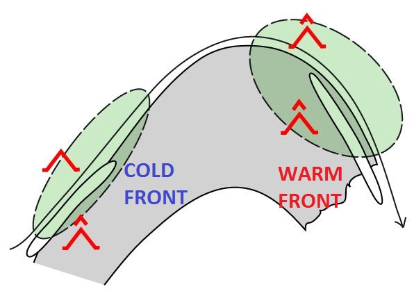
Fig. 3.1: Conceptual model of jet fibres [SatManu]
It has been observed that jet fibres are mostly found over warm front shields or behind a cold front.
Jet fibres are high altitude cirrus clouds with no connection to the surface weather. However, as they occur along the jet streak, jet-related phenomena such as turbulence can be expected in that region.
Turbulence generally occurs in a zone of high horizontal and vertical wind shear around the jet streak. Furthermore, a sharply curving jet stream on the poleward side of a warm front shield is associated with greater turbulence than a straight jet stream behind a cold front.
Figures 3.2 and 3.3 show jet fibres in the Dust RGB. Thin, high level ice clouds such as jet fibres appear black in this RGB combination, and can be distinguished from thick clouds, which appear red.
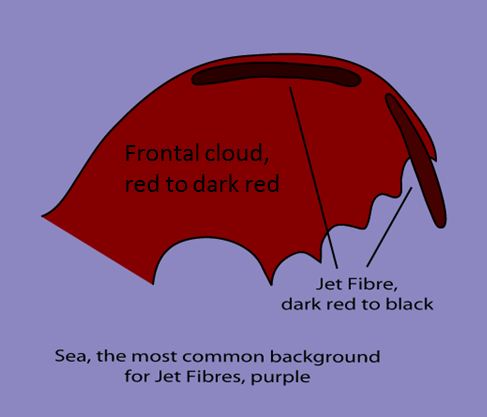
Fig. 3.2: Jet fibres in the Dust RGB [SatManu]
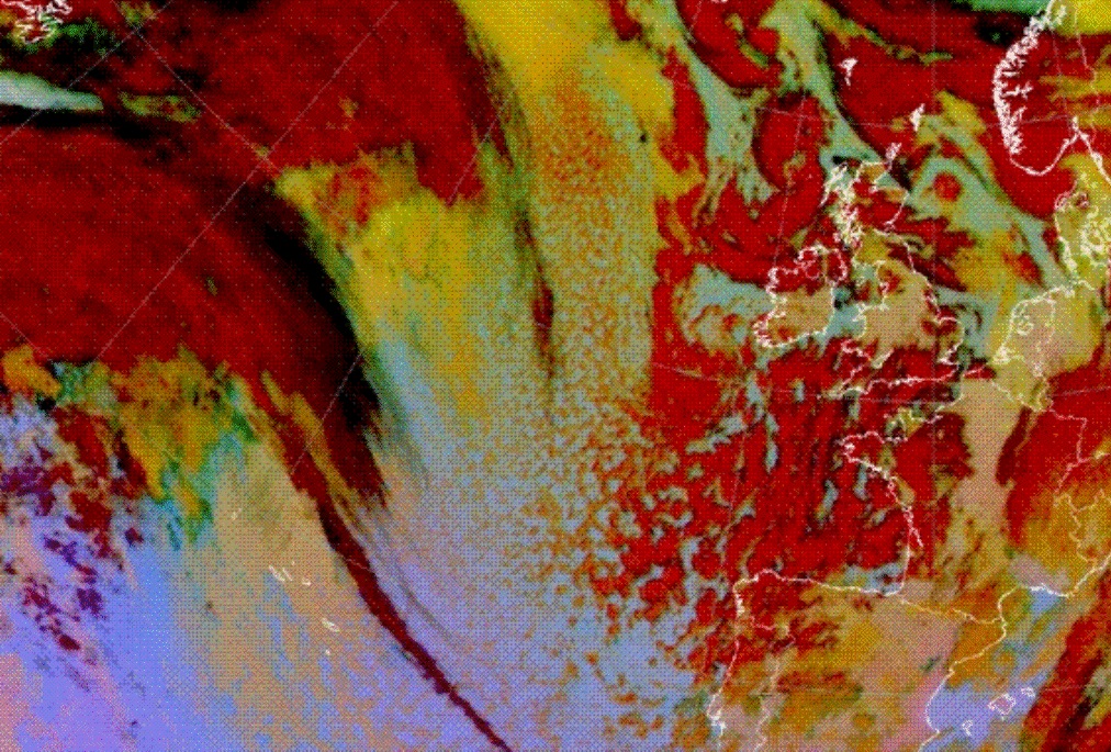
Fig. 3.3: 20 January 2009, 06 UTC, Meteosat 9, Dust RGB
When a fiber appears above a lower-level cloud feature, the cloud texture is different, which makes the fiber distinct from its surroundings. Jet fibres can appear anywhere jet streams are found, but they are easier to detect above the sea than over land because they contrast more strongly against the sea surface. In most cases jet fibres persist for 8 to 12 hours.
Please see the Manual of Synoptic Satellite Meteorology (SatManu) for more details on Jet Fibres .
Jet fibres in a case from 1 March 2008
On 1 March 2008 the synoptic situation was characterized by a rapid cyclogenesis over the Atlantic. At 15 UTC, a line of convective clouds reached the north of Italy. A jet stream with a maximum of 180 kt extended from Scotland to western Germany.
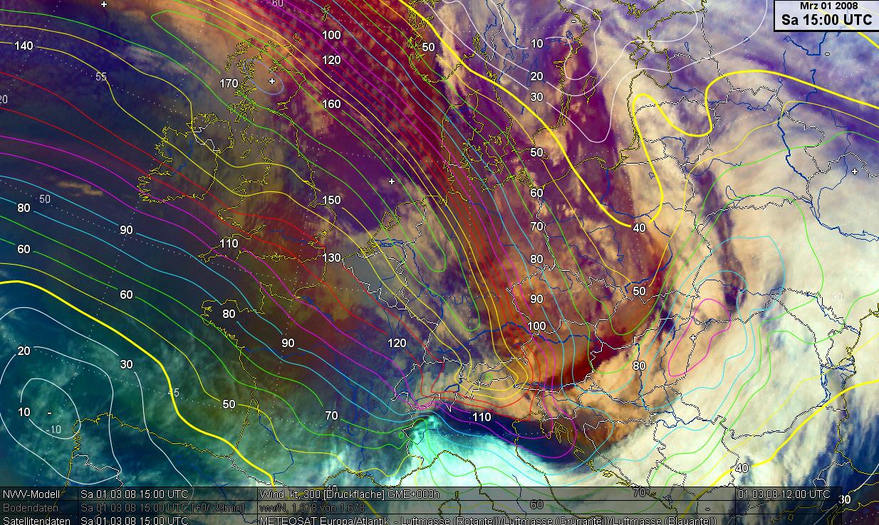
Fig. 3.4: 1 March 2008, 15:00 UTC. 300 hPa isotachs in kt, Airmass RGB
The images in Fig. 3.5 3.8 show sections of 15 UTC RGB's over Germany. There are jet fibres parallel to the jet axis. The white color in the Airmass RGB hints at high clouds. The HRV RGB and the HRV shows clearly the shadows of lower clouds over eastern parts of Germany.
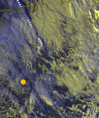
Fig. 3.5: HRV RGB [DWD] |
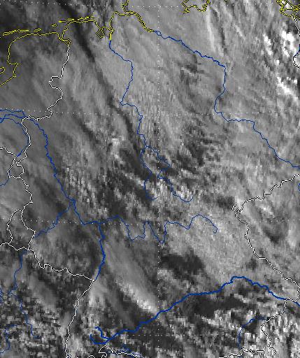 Fig. 3.6: HRV Fig. 3.6: HRV |
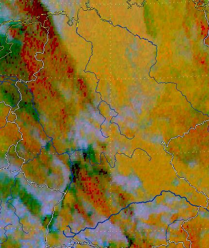
Fig. 3.7: Dust RGB [DWD] |
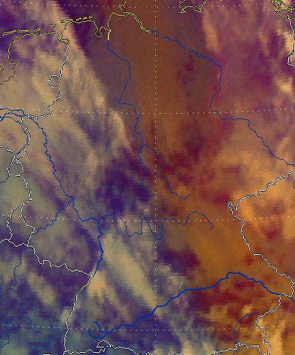 Fig. 3.5: Airmass RGB [DWD] Fig. 3.5: Airmass RGB [DWD] |
| (Fig. 3.5 3.8: 1 March 2008, 15:00 UTC [DWD]) |
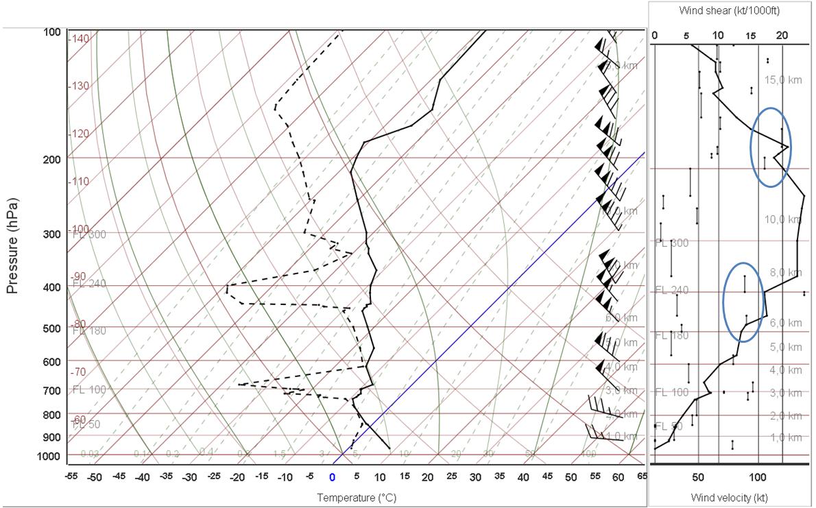
Fig. 3.9: Radiosonde Idar Oberstein, 1 March 2008, 18:00 UTC
Sounding on the left, wind velocity (kt) and shear (kt/1000 ft) on the right [DWD]
The radiosonde in Idar Oberstein (western Germany, yellow dot in the HRV-RGB) measured a maximum wind speed of 140 kt at a height of 10 km. Vertical wind shear in the jet core is around 15-20 kt/1000 ft.
You can use the vertical windshear for a useful empirical prediction of CAT.
If the vertical windshear is
≥ 6 kt/1000 ft, it is a hint for moderate CAT
≥ 9 kt/1000 ft, it is a hint for severe CAT
In this case, there is potential for severe CAT under and above the jet core (see the oval form).
Clear air turbulence behind a split cold front
For the 1 March 2008 case
The convective line of a split front moved southeast quickly. The corresponding images at 300 hPa reveal the convective line in the left exit region of the jet over central Europe. The convective line is just east of the trough's axis and southeast of the approaching PV-maximum at the level of potential temperature 310 K. The intense weather situation can be seen from the lightning detection chart (12942 strokes of lightnings within one hour, wind velocity of the lightning line about 100 km/h).
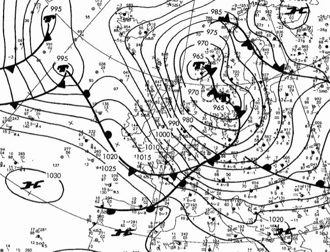
Fig. 3.10: Surface pressure, synop-observations and surface fronts, 1 March 2008, 06:00 UTC [DWD]
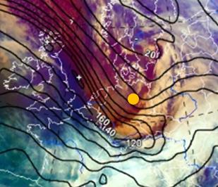
Fig. 3.11: Airmass RGB and Isotachs 300 hPa |
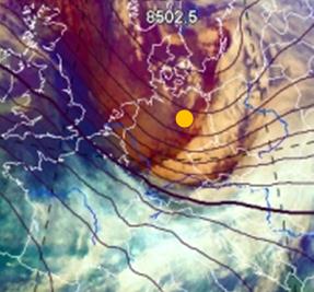 Fig. 3.12 Airmass RGB and Isohyps |
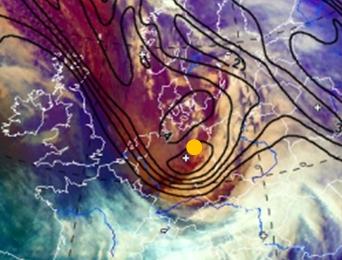
Fig. 3.13: IPV 310 K and Airmass RGB |
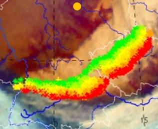 Fig. 3.14: Lightnings during last hour |
| (Fig. 3.11 3.14: 1 March 2008, 0900 UTC) |
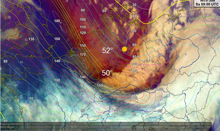
Fig. 3.15: 1 March 2008, 09:00 UTC, Airmass RGB, isotachs 300 hPa [DWD]
Question
You can use horizontal wind shear data to make a forecast of CAT for the area around Magdeburg.
If the horizontal windshear is
≥ 20 kt/deg of latitude, it is a sign of moderate CAT
≥ 30 kt/deg of latitude, it is a sign of severe CAT
Based on horizontal wind shear alone, would you expect severe CAT (see Fig. 3.15)?
The correct answer is a).
In the area of Magdeburg we only have a shear of 20 kt/one degree latitude (ca. 110 km).
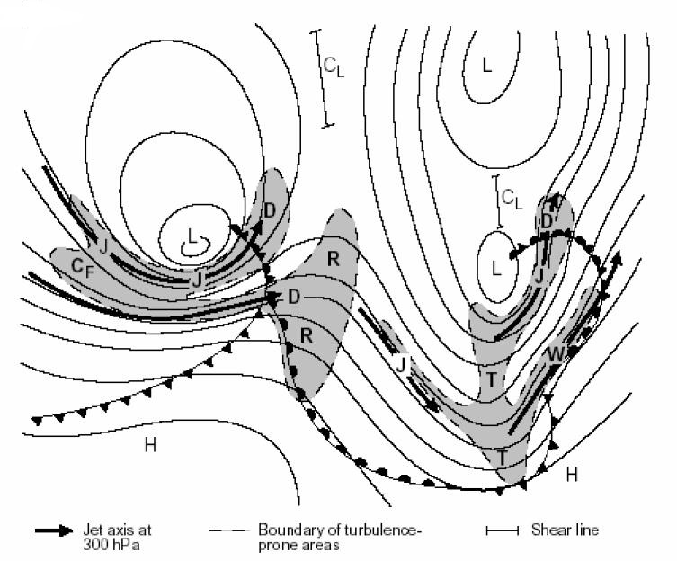
Fig. 3.16: Schematic showing analysis of 300 hPa geopotential and areas prone to CAT [WMO Aviation Hazards]
Question
In Fig. 3.16 you see an analyzed weather chart, with areas prone to CAT colored gray.
Which potential CAT areas in Fig. 3.16 do you find in the situation of Magdeburg (yellow dot in Fig. 3.11 3.15)?
The correct answer is b).
Explanations:
· T: This is not a really sharp upper trough.
· D: This is correct. There is wind shear in the diffluent exit region of the jet.
· J: This area is on the low pressure side of the jet, but there is no wind shear just inside the jet streak.
Until now, we have two signals for CAT in the area of Magdeburg.
The conceptual model of a split cold front can also indicate the presence of CAT. Behind the line of convective clouds there is a high risk of CAT due to
- descending dry air causing potential instability
- a transition zone from ascending to descending air
- the rapid movement of the front
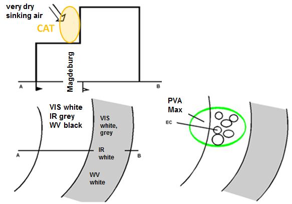
Fig. 3.17: Conceptual model of a split front
See the Manual of Synoptic Satellite Meteorology (SatManu) for more details Split Front.
Transverse bands and billows
Aircraft flying through transverse bands will cross volumes of air that are moving vertically at different speeds. Often there are features in the satellite images that suggest the presence of CAT, although its altitude cannot be determined accurately.
A characteristic pattern of cirrus clouds, known as billows, signals the presence of CAT. Billows are an indication of a turbulent flow described by the Kelvin-Helmholtz instability
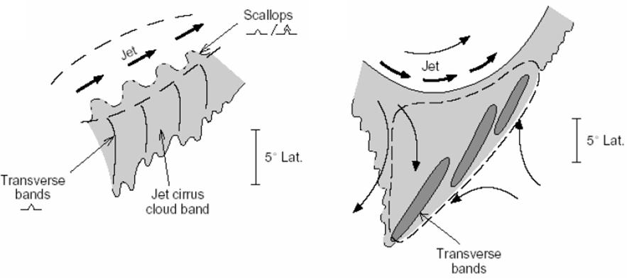
Fig. 3.18: Conceptional Model of Transverse bands and Scallops [WMO Aviation Hazards]
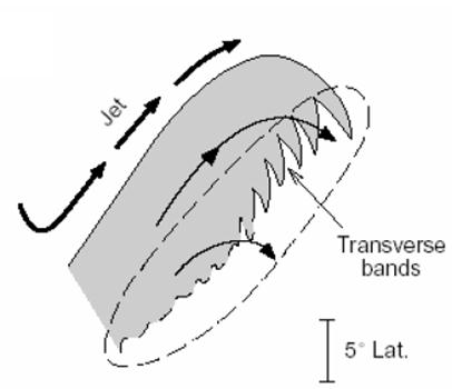
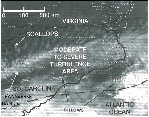
Fig. 3.19a (left): Conceptional Model of Transverse bands [WMO Aviation Hazards]
Fig. 3.19b (right): Satellite image with Transverse Bands, Scallops, Billows [WMO Aviation Hazards]
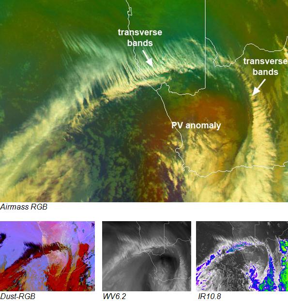
Fig. 3.20: 9 November 2009, Eumetsat Image Gallery: Transverse bands over South Africa and Namibia [EUMETSAT]
The Airmass RGB, Dust RGB, WV6.2 and IR10.8 channel images above give examples of transverse cirrus bands. Large transverse cirrus bands can be seen over southern Namibia and smaller ones over the central parts of South Africa. Since there are few airplane observations from southern Namibia or the northwestern part of South Africa, it is difficult to verify whether there was turbulence in the area of the transverse cirrus bands or not. [from Jochen Kerkmann, Eumetsat]
See the loop of this Airmass RGB from 9 November 2009
Question
Locate the jet stream in this Airmass RGB by clicking on it.
Question
Which particular cloud formation signals potential clear air turbulence?
The correct answer is a), b), c), and d).
All 4 cloud formations give you a signal for potential Clear Air Turbulence.
Clear air turbulence near billows and lee clouds
A characteristic pattern of cirrus clouds are billows. Often they are a strong signal for CAT. The billows are an indication of breakdown into turbulent flow in the form of Kelvin-Helmholtz instability. Then reason is velocity shear in the air. Have a look at this numerical simulation.
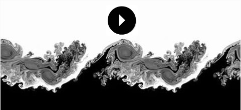
Animation 3.22: Numerical simulation of a Kelvin-Helmholtz instability [Wikipedia]
Note that even in the stratosphere, where static stability is high, turbulence and breaking waves can still be generated if the wind shear is strong enough. Values of Richardson number Ri (the ratio of potential to kinetic energy) less than 0.25 will allow the production of breaking waves. Values between 0.25 and 1.0 will allow turbulence to persist, whereas values greater than 1.0 will tend to cause any existing turbulence to subside. [WMO Aviation Hazards]
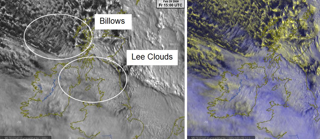
Fig. 3.23: HRV Fig. 3.24: HRV RGB
Fig. 3.24: HRV RGB
Both images: 29 Feb 2008, 15:00 UTC [DWD]
In the HRV RGB, we see (bluish) billows embedded in a very strong airflow over the yellow low clouds. There is a combination of billows and lee clouds over Great Britain and Ireland.
Mountain wave activity is often very apparent in satellite imagery. Trapped waves are often easily diagnosed, with very clear wave-like patterns in both infrared and visible imagery. Untrapped, or vertically propagating waves, are often indicated by orographic cirrus cloud features. In the figures above it is difficult to differentiate between the billows and lee clouds.
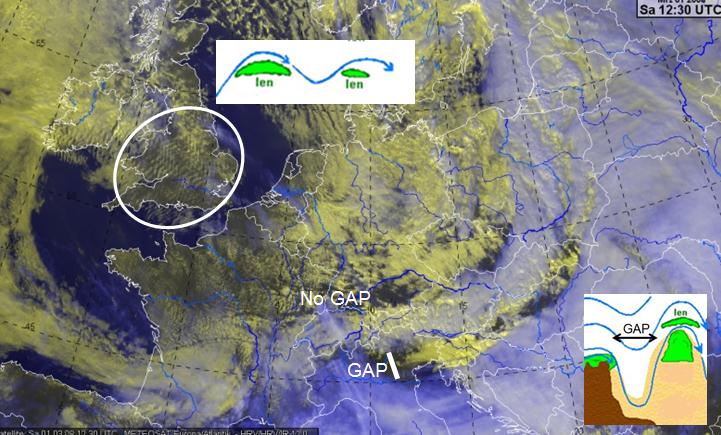
Fig. 3.25: 1 March 2008, 12:30 UTC, HRV RGB [DWD]
Lee waves generate lenticularis clouds over England and south of the Alps.
The circled area contains lee waves. Due to the strong winds, there is a high probability of clear air turbulence over these clouds.
Another sign of CAT is the gap between the mountain ridge and the thick cold cirrus clouds, caused by the strong wind shear. These clouds are bluish in the HRV RGB.
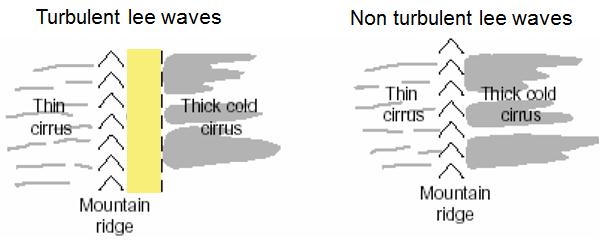
Fig. 3.26: The gap can be a sign of CAT [WMO Aviation Hazards]
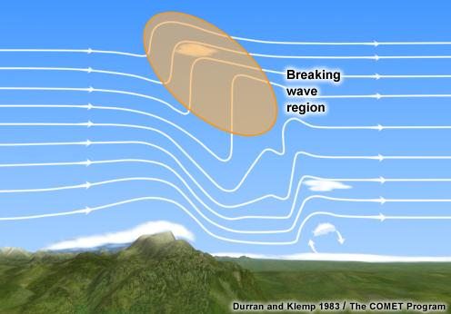
Fig. 3.27: Breaking wave region [COMET]
The gap is often a sign of vertically propagating waves of considerable amplitude. They may break in the troposphere or lower stratosphere. Wave-breaking can result in severe to extreme turbulence in that region and nearby. This typically occurs between FL200 and FL400 (6000 m – 12000 m). If a vertically propagating wave does not break, an aircraft would likely experience considerable vertical sway, but little turbulence.
In some cases of strong lee waves there is not enough moisture in the air for visible clouds to form. However, the lee cloud tops might be still seen in the Airmass RGB. They are easiest to see with polar orbiting satellites with a device for detecting water vapor, such as MetOp.
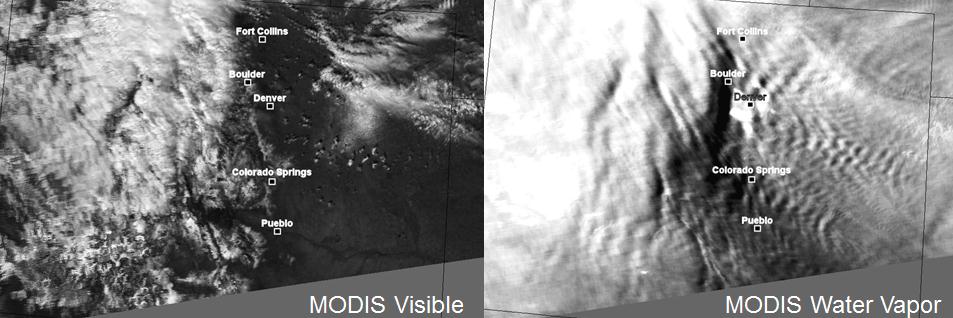
Fig. 3.28: Lee Waves without condensation in VIS and WV image [Wayne Feltz]
Clear air turbulence near deep convective clouds
It should be noted that transverse cirrus bands with a hint of clear air turbulence can also be observed above or around deep convective clouds. An example is described in the case study of 25 May 2009. In the morning of that day, Meteosat observed an interesting convective system over Northern France, with strong overshooting tops, a high-level plume and radial cirrus clouds. The Meteosat-8 rapid scan loop (HRV channel) from 6:00 to 7:00 UTC shows the high-level plume and the radial cirrus clouds. Gordon Bridge, who was flying through the area of radial cirrus clouds from London over Belgium to Frankfurt (see marked line in Fig. 3.29) noted some moderate turbulence at around 35.000 ft in the vicinity of Brussels, which interrupted the serving of refreshments for a short while. This moderate turbulence could well have been what is called "convectively induced turbulence".
The following image shows some of the wave structures, but MSG SEVIRI has too coarse a resolution to detect the smaller waves (less than 5 km wavelength), which are visible in MODIS images.
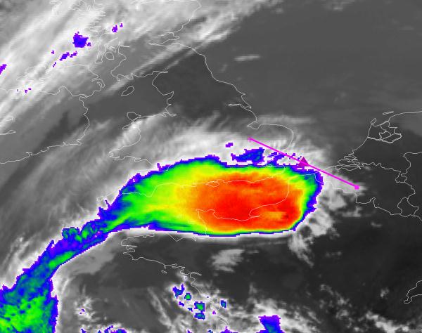
Fig. 3.29: 25 May 2009, IR10.8, 06:45 UTC. Particular wave structures [EUMETSAT]
This case of deep convection contains a very good example of gravity waves. If wind shear is weak, gravity waves look like concentric ripples. In the presence of strong wind shear, the waves can break (KelvinHelmholtz instability) and cause clear air turbulence.
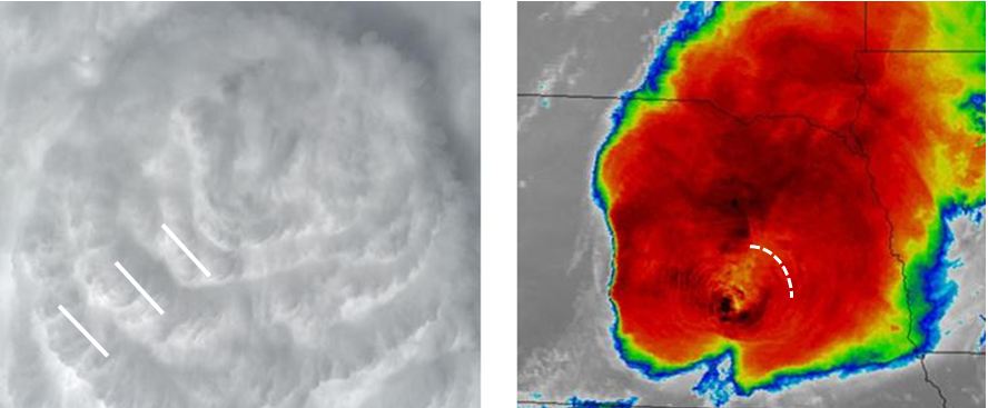
Fig. 3.30: Gravity waves on top of thunderstorms [Pao K. Wang, Wisconsin]
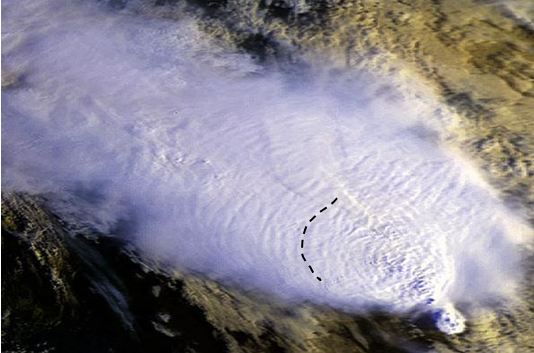
Fig. 3.31: Gravity waves on top of thunderstorms [Pao K. Wang, Wisconsin]