Forest Fires

Up until now we have discussed the synoptic patterns that play a role in forest fires and slowly zoomed in to discuss which atmospheric features are associated with forest fires.

In this chapter we will zoom out again, to 35.787 kilometres to be exact, as we will discuss and show how Meteosat Second Generation is suited for detecting and monitoring wild fires. As you will see, this is of great importance, especially in remote areas.

Radiation Laws and Hot Spots

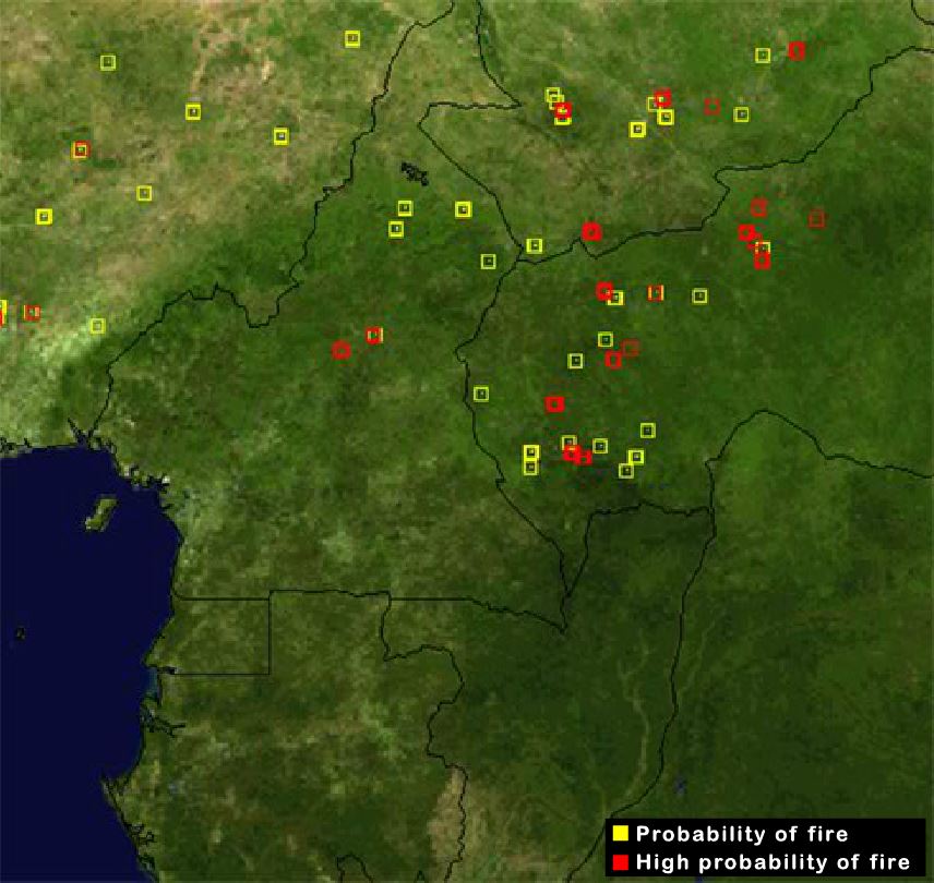
Fig5.1 - EUMETSAT MPEF fire product for Meteosat 9 over central Africa on 22 January 2008 at 14 UTC. "Probability of fire" in yellow squares and "high probability of fire" in red squares.

Figure 5.1, obtained from Meteosat 9 at 14 UTC on 22 January 2008, shows the locations of probable fires over Central Africa. Yellow squares denote a lower probability and red squares a higher probability for fires.

The algorithm behind this product uses bands of 3.9 μm and 10.8 μm in the thermal infrared region of the spectrum. To understand why these bands are used, you must first recall the Planck law for black body radiation and the Wien displacement law of radiation.

Did you know?

The 3.9μm channel is not solely a thermal channel. The signal in 3.9μm channel is a combination from reflected solar and emitted thermal radiation!

Planck's Law

Planck's law gives the amount of electromagnetic energy radiated by a black body for different wavelengths in thermal equilibrium.

Fig 5.2 - Black body spectrum.

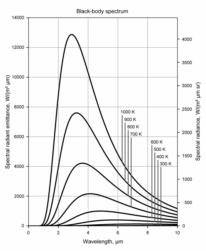
Bodies at different temperatures have different curves, with a steep rise of irradiance on shorter wavelengths and a long descent on longer wavelengths (Figure 5.2).

Wiens' Law

Plancks' law was an attempt to improve upon an expression proposed by Wilhelm Wien (Wien's law) which fit the experimental data at long wavelengths but deviated from it at short wavelengths.

Wiens' displacement law states that there is an inverse relationship between the wavelength of the peak of the emission of a black body and its temperature (Fig. 5.3).

Fig 5.3 - Black body spectrum with peak emission indicated with red dashed line.

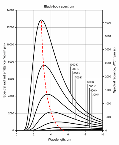
To summarize, Wiens' displacement law shows that the hotter an object is, the shorter the wavelength at which it will emit most of its radiation.

The sun is a reasonably good approximation of a black body with a temperature of 5777 K. Using Wien's law, this temperature corresponds to a peak emission at a wavelength of 0.5 μm (visible region of the spectrum). On the other hand, many parts of the Earth's surface may be considered a black body at temperatures of 280 K, for which the maximum spectral radiance occurs at a wavelength of 10.35 μm, corresponding to the thermal infrared region of the spectrum.

Fig 5.4 - The wavelengths corresponding to the peak emissions of the Sun (5777 K; orange) and Earth's surface (300 K; red).

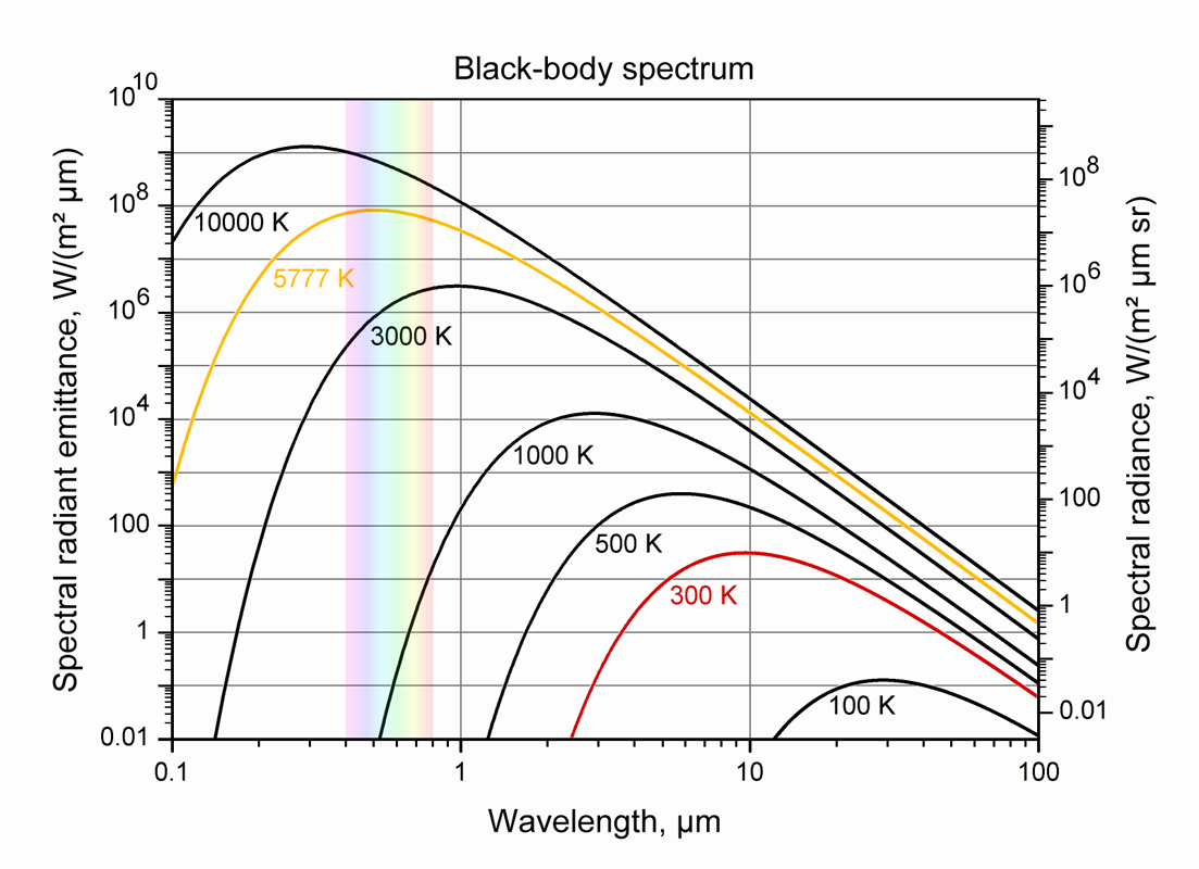
Figure 5.4 shows the Planck curve for black bodies at 5777 K and 300 K (close to the Sun and Earth's "black body" temperatures).

Due to the huge disparity between the radiation and wavelength ranges occuring at temperature values of 6000 K and 300 K, logarithmic scales are more appropriate for depicting the two curves shown.

Fig 5.5 - The wavelengths corresponding to the peak emissions of the Sun (5777 K), the Earth's surface (300 K) and forest fires (600 to 1000 K).

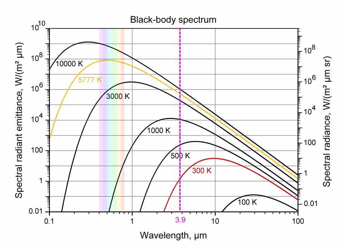
If you look carefully at Figure 5.5 you will get a hint as to why the channel 3.9 μm onboard Meteosat Second Generation is suitable for detecting and monitoring forest fires.

The dashed line represents the 3.9 μm band and you see from Wien's law that 3.9 μm is the wavelength at which a blackbody at 743 K has its peak. Obviously, this temperature corresponds to the temperature of a fire!

This is one reason why the IR3.9 channel is suitable for detecting and monitoring forest fires, but there are more reasons.

Temperature Responsivity

Bands around 3.9 μm are also suitable for detecting fires because of two other properties: Temperature responsivity and Sub-pixel response.

Temperature responsivity results from the fact that the Planck function is not linear. In fact, it can be demonstrated that radiance (B) can be related to temperature (T) by the following expression:

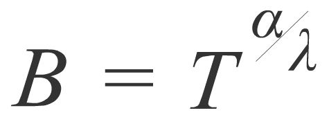
where α is a constant (approx. 2.8214) and λ is the wavelength. Please note that this is an approximation derived from the Planck law (the so-called Rayleigh-Jeans approximation) and is good to about 1% for long wavelengths, and therefore applicable to normal ground temperatures and fire temperatures.

So, temperature responsivity states that for different wavelengths, the change of radiance with respect to change in scene temperature varies as T is raised to the quotient of the constant α divided by the wavelength λ, the change in scene temperature is thus much larger at shorter wavelengths!

To explain the concept of "temperature responsivity" graphically, let us look to three Planck curves for black bodies at terrestrial temperatures (260, 280 and 300 K).

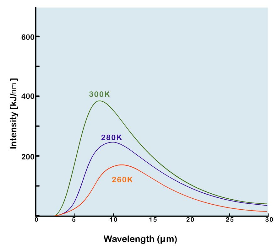
We zoom in on the 10 μm region of the spectrum and consider the change in intensity between the three curves.

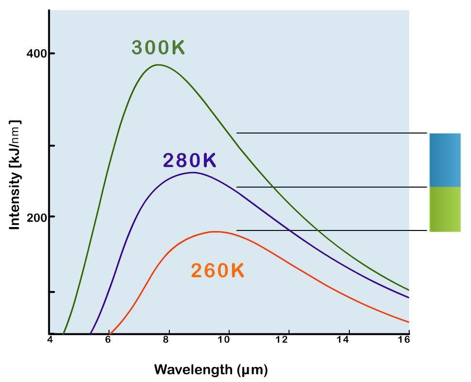
At 10 μm a temperature change from 280 K to 300 K (blue bar) yields a change in intensity slightly larger than the change in intensity from 260 K to 280 K (green bar)!

However, if we zoom in on the region around the 4 μm region of the spectrum, the relative change of intensity is much larger at higher temperatures (blue bar) than at lower temperatures (green bar)!

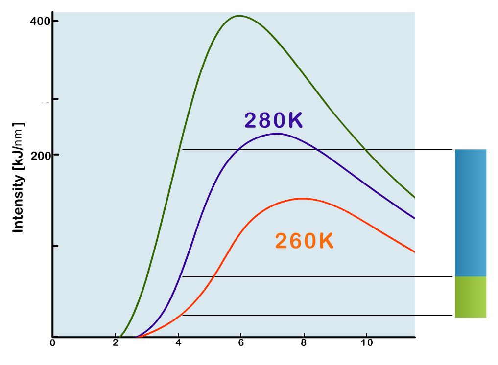
This simply means that a change in scene temperature due to a fire will show a greater response at 4 μm than at 10 μm!

Sub-pixel Response

Another reason why the band around 3.9 μm is more capable of detecting fires is because of a process called "Sub-pixel response".

Imagine a fire occupying the whole pixel on a clear dry night (no clouds and no solar radiation). In this case, the temperature across the pixel would be approximately uniform and we should expect the same radiance temperature at the 3.9 μm and 10.8 μm bands! In this case, it would not be possible to identify a fire pixel by comparing the two bands.

Luckily, the fire front does not occupy the entire pixel. First, this is good because a large forest area is not being burned all at once! Second, this is the way to detect a fire through satellite remote sensing!

Basically, the concept of sub-pixel response states that if there is variability within a field-of-view (FOV), then the radiance measured by the satellite for that FOV is the average of the individual radiances in the sub-pixels and not of their temperatures.

In this example over Portugal we have one MSG SEVIRI pixel which is divided into four sub-pixels. Among these sub-pixels we find a "hot spot" of 500 K. Using Rayleigh-Jeans law (5.1.3) we can then calculate the following brightness temperatures (BT) for the MSG SEVIRI pixel for the IR10.8 and IR3.9 channels.

You see that in a pixel partly covered by a fire, the radiance at 3.9 μm is larger than at 10.8 μm due to the stronger response at 3.9 μm to the warmer portion (fire) inside the pixel. In fact, EUMETSAT´s algorithm shown at the beginning of this chapter uses the temperature difference IR3.9-IR10.8 (different temperature ranges for day and night) as a proxy for fire probability - the larger the difference, the higher the probability!

The EUMETSAT algorithm also includes thresholds for pixel radiances at 3.9 μm and for the standard deviation of radiances over 3x3 pixel boxes at 3.9 μm and 10.8 μm. The standard deviation at 3.9 μm is used to split small fires from large hot fires and the standard deviation at 10.8 μm is used to discard inhomogeneous land or clouds previously undetected in a cloud mask.

Hot Spots Gallery

In this section we will show you a gallery on how remote sensing helps to detect hots spots.

Fig. 5.7 - Meteosat 8 IR3.9 - 25 July 2004 17:15 UTC.

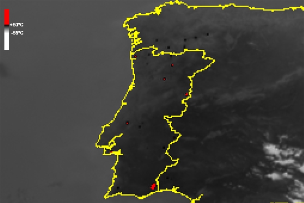
This Figure is an example of an IR3.9 image over Portugal and part of Spain, with hot spots in red, where the brightness temperature exceeds the threshold of 50 ºC.

Fig. 5.8 - Meteosat 8 IR3.9 - 4 August 2005 13:00 UTC.

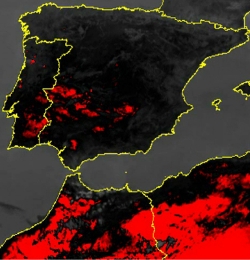
Although it may seem a promising image for detecting fires, in fact it does not distinguish fires from hot land during the day as we see in the this example of a hot summer day (Fig 5.8).

Fig. 5.9 - Left image: Meteosat 8 IR3.9 - 3 August 2003 12:00 UTC (inverted grey scale - hot spots as darker pixels). Right image: Meteosat 8 NIR1.6 for the same instant (non-inverted grey scale - hot spots as white pixels). Click to enlarge.

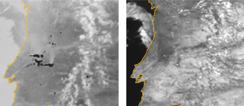
Two Meteosat 8 images are shown here. On the left there is the 3.9 µm (inverted image) and to the right the near-infrared 1.6 µm. Most striking in the 3.9 µm image are the hotspots associated with the fires (darker pixels). A closer look even reveals some smoke swirling northward from those pixels. If fires are too hot they may even be detected using 1.6 µm. In this example, only a few pixels with high radiance values (white pixels) are identified at 1.6 µm, while the number of pixels in the 3.9 band is much larger (number of dark pixels). Note the hot spot color is different in the images, as the IR3.9 is inverted and the NIR1.6 is not!

Fig. 5.10 - Meteosat 8 Night Microphysical RGB - 5 August 2005 02:00 UTC. Pixels are depicted in magenta for fire hot spots. Source: Portuguese Met. Service.

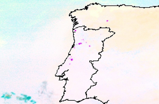
Figure 5.10 shows the so-called Night Microphysical RGB where the range and gamma values are defined to depict fire pixels in magenta.

The magenta color results from high values on the red and blue beams and low values on the green beam. The key beam is in fact the green - less and less green is obtained when IR3.9 brightness temperature increases and steps away more and more from the IR10.8 brightness temperature (up to a maximum difference of 15 ºC). Also, the air has to be very dry, so the difference between the brightness temperatures of IR10.8 and IR12.0 is close to 0 (maximum of red), and the fire pixels have to have a brightness temperature of at least 20 ºC in IR10.8 (maximum of blue). These two final conditions are peanuts for a fire event, right?

Fig. 5.11 - Meteosat 8 IR3.9 - 21 August 2005 17:00 UTC.

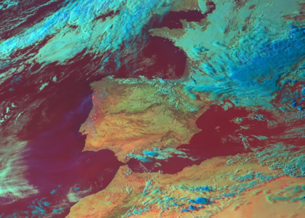
In Figure 5.11 one can see the construction of the so-called Fire RGB which uses the VIS0.6, HRV and IR3.9 channels. In the ultimate RGB the fires themselves appear as red dots. A close look also shows the smoke which was swirling over the Atlantic Ocean on that day.

During the night there is no contamination of the IR3.9 band by solar radiation. Naturally, this is not the case during the day, which makes it more difficult to detect hot spots. However, there have been case studies where some RGBs have been successfully used to detect hot spots subjectively during the day. The image shows the hot spots over northern and central Portugal on a day during the devastating 2005 forest fire season.

Fig. 5.12 - Left Image: Meteosat 8 IR3.9 - 7 July 2003 (inverted grey scale - hot spots as darker pixels). Right Image: Meteosat 8 IR3.9-IR10.8 - 7 July 2003 (the brighter the pixels the higher the difference). Click to enlarge.

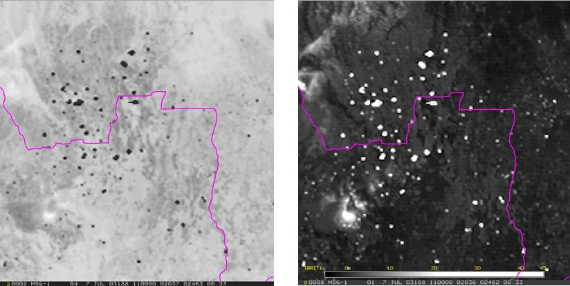
Here is a case of fire hot spots over Congo and Angola. The fires are depicted in both the single IR3.9 image and the difference IR3.9-IR10.8 image.

Fig. 5.13 - Metop AVHRR RGB composite channels 1, 2, 3 - 25 August 2007 09:55 UTC.

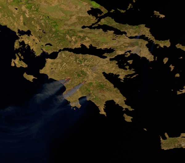
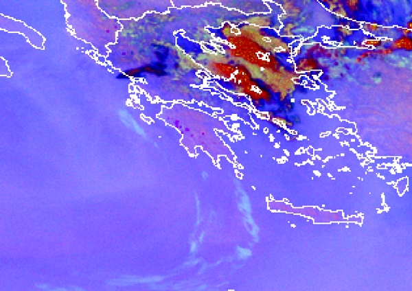
The following two examples are from Greece during the last week of August 2007, when large parts of the Greek countryside - from the island of Evia north of Athens to the Peloponnese in the south - were ravaged by some of the worst wildfires in living memory.

The locations of fires and smoke can also be seen with the METOP satellite using the AVHRR instrument.

Fig. 5.14 - Meteosat 9 Night Microphysics RGB (IR12.0-IR10.8, IR10.8-IR3.9, IR10.8) - 26 August 2007 03:00 UTC

Another RGB image which uses most of the thermal channel (which makes it possible to also monitor fires at night). The hot spots themselves are seen as small red dots in the center of the image.

Fig. 5.15 - EUMETSAT MPEF fire product for Meteosat 9 over Central Africa on 10 July 2008 12:15 UTC. Probability of fire in yellow squares and high probability of fire in red squares. Updated daily.

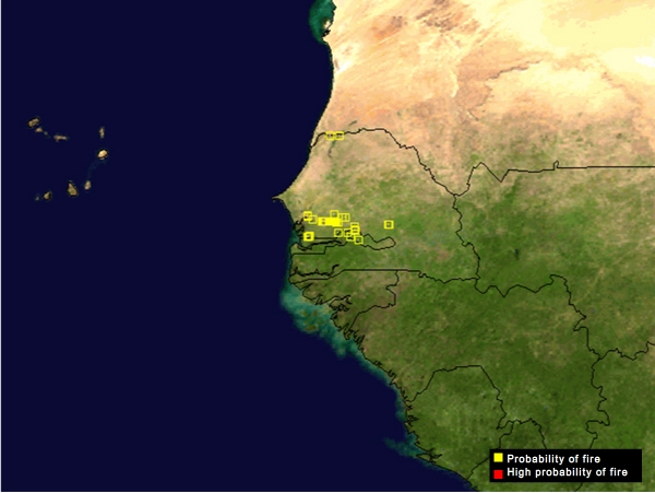
Figure 5.15 is again the EUMETSAT fire product which was also presented in the beginning of this chapter. In this case a zoom is made over western Africa, where pixels with a probability of fire are found over Senegal and Gambia during the summer of 2008.

Fig. 5.16 - Composite of LSASAF Fire Detection & Monitoring (FD&M) product for January 2007. Courtesy of LSA-SAF.

The Fire Detection & Monitoring product from the LSA SAF (Fig. 5.16) is a pre-operational procedure that allows detecting active fires based on information from MSG-SEVIRI. The procedure takes advantage of the temporal resolution of SEVIRI (one image every 15 minutes), and relies on information from SEVIRI channels (namely 0.6, 0.8, 3.9, 10.8 and 12.0 μm) together with information on illumination angles. The method is based on heritage from contextual algorithms designed for polar, sun-synchronous instruments, namely NOAA/AVHRR and MODIS/TERRA-AQUA. A potential fire pixel is compared with the neighbouring ones and the decision is made based on relative thresholds as derived from the pixels in the neighbourhood.

Fig. 5.17 - MODIS fire product (polygons in red) on 25 September 2007 over Bolivia. Source: NASA Earth Observatory - Natural Hazards.

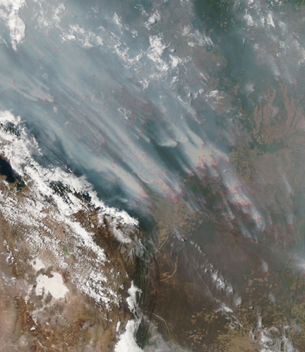
Hundreds, possibly thousands of fires (locations marked in red) were burning in South America when the Moderate Resolution Imaging Spectroradiometer (MODIS) on NASA's Aqua satellite passed overhead on 25 September 2007 and captured this image. The most intense fire activity was in Bolivia, where fires are concentrated in the Santa Cruz Department, in the southeastern part of the country. Thick smoke hangs over much of the scene. The towering Andes mountains (lower left) partially block the flow of smoke to the west.

Fig. 5.18 - MODIS fire product (polygons in red) on 8 July 2008 over Turkey and Cyprus. Source: NASA Earth Observatory - Natural Hazards.

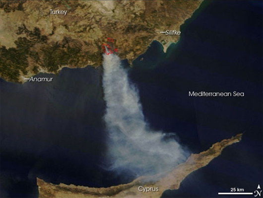
The MODIS fire product mentioned earlier is very well suited for the detection of hotspots in a higher resolution than those obtained from geostationary platforms such as the MSG. This is an example of the MODIS fire product in southern Turkey, in which the hotspots are plotted in red polygons. These are superposed on a composite image using three bands from the visible region of the spectrum. In the image, the smoke generated by the fire is also clearly visible as it is being driven southward and reaches Cyprus.

Although it might be easier to identify small/weak forest fires with a polar orbiter satellite, like is the case of MODIS, the high temporal frequency provided by geostationary observations enables to follow the life cycle of the identified fires. An example of this is provided by fig. 5.19 showing the temporal behaviour of the wild fires over the Sahel region for 2 weeks in 2004 as captured by a fire product derived from Meteosat 9, the Fire Radiative Power (in short, FRP) (on the left axis). This product is also being computed by the LSA SAF. As you can see, the temporal behaviour of the fire activity is very well captured by the high SEVIRI revisiting time (15 minutes). The colors represent different land covers; Mosaic Forest, Savanna and Deciduous woodland have the most pronounced diurnal cycle of the fire activity.

Fig. 5.19 - Daily variations of the FRP (Fire Radiative Power produced by the LSA SAF) and the combustion rate over the Sahel region, averaged from 1 to 15 February 2004. (In: Yves Govaerts et al., The operational MSG/SEVIRI fire radiative power product generated at the LAND SAF. Proceedings of 2008 EUMETSAT Meteorological Satellite Conference, Darmstadt, Germany, 8 - 12 September 2008). Click to enlarge.

The previously mentioned Fire Radiative Power (FRP) product from LSA SAF corresponds to the amount of radiant heat energy of a fire per unit time. It is measured in megawatts every 15 minutes on a pixel basis, being currently in a pre-operational status. The example showed in Figure 5.20 is for the fires over Greece on 25th August 2007 at 09:45 UTC. Note that this product can be extremely useful as it was found to be related to the amount of fuel consumed by fires.

There is another related product that will become available in 2012: the FRP grid, which will estimate hourly averages of FRP within 1º longitude times 1º latitude boxes. The FRP grid will also benefit from a correction for small fires that go undetected by SEVIRI and for potential cloud contamination. These corrections are based on statistical analysis performed for each box and the user will access both the end product and all correction factors applied. Other main ancillary pieces of information stored in the product include the percentage of burnt area and the average number of detected fires per grid box.

Fig. 5.20 - Fire radiative power on 12 October 2011, derived from SEVIRI (LSA SAF) and MODIS (NASA) data averaged over 125 km grid cells [mW/m2], for the MACC (Monitoring Atmospheric Composition & climate) D-Fire subproject. Click to enlarge.

Figure 5.20 presents the thermal radiation coming from actively burning vegetation and other open fires for 12 October 2011. The data is derived from SEVIRI (LSA SAF) and MODIS (NASA) and calculated as daily averages of FRP in 125 km grid cells [mW/m2]. This (daily average) FRP areal intensity data is computed within the D-Fire subproject, which provides data of global emissions from biomass burning that are used as model input for smoke distribution forecasts (organic matter, black carbon and sulfate aerosols). The emissions are calculated in real time and retrospectively from satellite-based observations of open fires (for example wildfires and human-ignited grassland and forest fires).

Fig. 5.21 - Modelled organic matter plus black carbon AOD [-] (left, blue) and MODIS visual images (right) for an Aqua overpass on 25 August, 12:05 UTC, (top) and a Terra overpass on 26 August, 09:35 UTC (bottom). Overlaid with SEVIRI FRP [W/m2] interpolated to model resolution (left, orange) and MODIS hot spots in (right, red). Click to enlarge.

The left panel shows the fire intensity observed by the SEVIRI instrument in terms of fire radiative power (FRP per unit area at 25 km resolution, reddish color bar) and the optical depth of the simulated resulting smoke aerosols (AOD, bluish color bar) for 26 and 27 August. Images on the right show concurrent MODIS observations; the simulations and observations of the Greek fire plumes display very similar shapes. (source: landsaf.meteo.pt)

Aerosols

Throughout this module you have seen several images of fires. Some of them included data from bands in the visible part of the spectrum, in which fire smoke and resulting clouds (pyrocumulus) could be easily detected. In this section we will briefly address the principles that are behind the images, meaning the properties of the aerosols that result from forest burning, which are also frequently referred to as biomass burning aerosols. Note that aerosol chemistry and the physics related to biomass burning are currently active topics of research in climate models, but we will leave this topic for you to look into in case you are interested.

Aerosol Detection

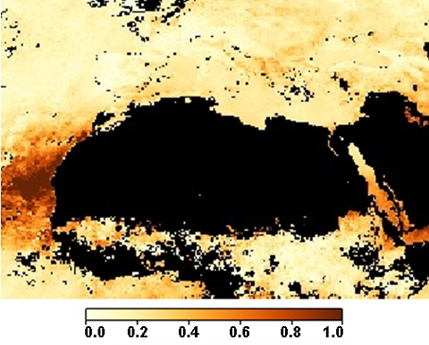
First you should be aware that the channels best suited for aerosol detection are those with wavelengths smaller than 0.7 μm (700 nm), because there is less reflectance from the surface (forest, types of soil, ...) to interfere in the detection. You can check this property in Figure 5.22, which shows the difference of soil reflectance and (mainly) leaf reflectance between the two SEVIRI visible narrow bands (0.6 μm and 0.8 μm).

Fig 5.22 - Reflectance from leaves (green curve) and soil (orange curve) in the visible and near-infrared region of the spectrum, as sensed by four SEVIRI channels: 0.6, 0.8 and 1.6 μm (dark grey) and HRV (light grey). Top of the atmosphere (TOA) irradiance in red. Click to enlarge.

The aerosol optical thickness (or aerosol optical depth) is a measure of the concentration of aerosols in the atmosphere and can be estimated through remote sensing. The product is obtained with the MODIS sensor on board the AQUA and TERRA satellites. It is available on 10 km boxes for seven wavelengths between 0.47 and 2.13 μm over ocean and three wavelengths (0.47 μm, 0.66 μm and 2.13 μm) over land. A joint land and ocean product is estimated for 0.55 μm as this wavelength is usually used in climate modelling (Remer et al, 2005).

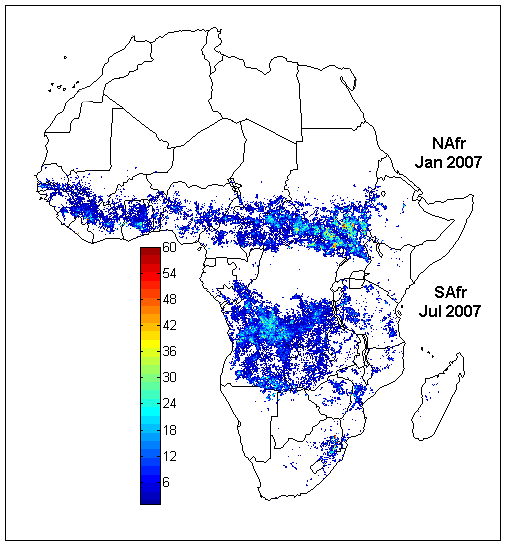
You can see an example in Figure 5.23 in which several local maxima are depicted for the period between 1 July and 1 August 2007.

Fig 5.23 - Aerosol Optical Thickness from the MODIS instrument on board the TERRA satellite for the period between 1 July and 1 August 2007 over southern Europe and northern Africa.

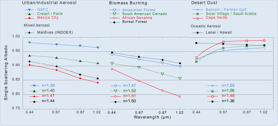
In fact, the absorption of radiation by biomass burning aerosols is higher than for other aerosols, such as desert dust or oceanic aerosols. This fact is confirmed in Figure 5.24, where single scattering albedo (ratio of scattering to scattering plus absorption) is shown for different kinds of aerosol; urban/industrial, biomass burning, desert dust and oceanic aerosol. The lower the single scattering albedo, the higher the absorption!

Fig 5.24 - Single scattering albedo for different kinds of aerosol - urban/industrial, biomass burning, desert dust and oceanic aerosol (Retrieved from Dubovik et al, 2002). Click to enlarge.

You should also keep in mind that for biomass burning, approximately 90% of released carbon is oxidized to CO₂ or CO and less than about 5% of the carbon is released as particulate matter. Furthermore, smoke particles (which are composed of both organic carbon [~50-60%] and black carbon [~5-10%]) are effective cloud condensation nuclei, therefore influencing cloud microphysics and even precipitation processes (Reid et al, 2005).

However, the relationship between aerosols and clouds (aerosol-cloud interaction) is not so straightforward as you may think. Studies for Brazilian forests show that a greater aerosol load leads to higher cloud droplet concentrations (or cloud fractions), but only up to a point. In fact, above a certain threshold, increasing aerosol load does not necessarily lead to more cloudiness (Feingold et al, 2001, Xue et al, 2008). For these cases, other properties may play a role, namely the size of the aerosol particles and the hygroscopicity (capacity of the aerosol to react with air moisture content), but this topic is still under investigation by the scientific community.

So, when you see smoke on an image using bands from the visible part of the spectrum, you may expect to also see water clouds after some time, including the so-called pyrocumulus we already had the opportunity to discuss earlier in the module.

Aerosol Gallery

We now show you some examples of smoke clouds, pyrocumulus clouds and other products of aerosols and gases. Some of the examples are similar to ones seen before, but you can now look at them from a different perspective!

Figure 5.25 - MODIS image from 29 July 2007 from NASA´s TERRA satellite. Source: NASA Earth Observatory - Natural Hazards.

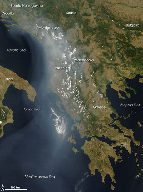
This first MODIS image taken on 29 July 2007 shows parts of Greece, Montenegro, Macedonia and Albania. Both fire smoke clouds and water clouds are seen in this image.

Figure 5.26 - MODIS image from 22 August 2007. Source: NASA Earth Observatory - Natural Hazards.

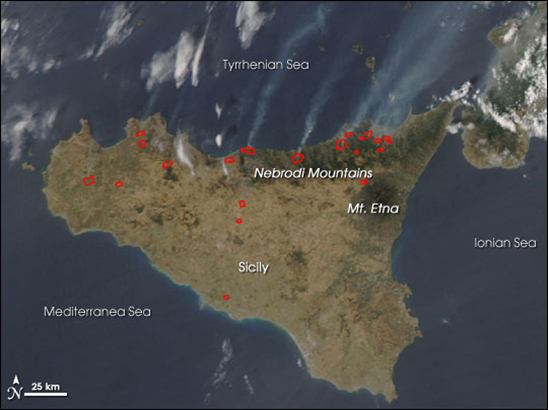
Smoke and fire product (polygons in red) over Sicily. The northward flow of the smoke indicates the wind direction clearly.

Figure 5.27 - MODIS image from 30 July 2007. Source: NASA Earth Observatory - Natural Hazards. Click to enlarge.

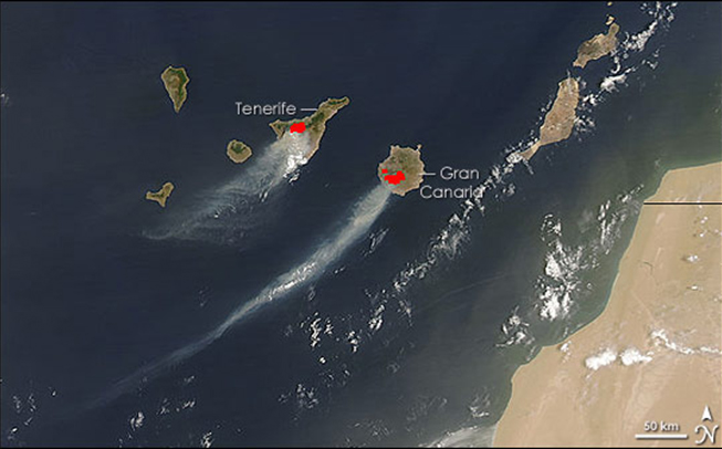
Smoke and fire product (polygons in red) over the Canary Islands in the Atlantic (namely Gran Canaria and Tenerife). A northeasterly flow over the Islands drags the smoke away from the fires. Note how there is a high contrast over sea and a low contrast over land, in particular in Tenerife.

Figure 5.28 - HRVIS RGB image (HRVIS; HRVIS; IR10.8) from Meteosat 8 on 20 July 2005 at 17:00 UTC. Source: Portugese Meteorological Service.

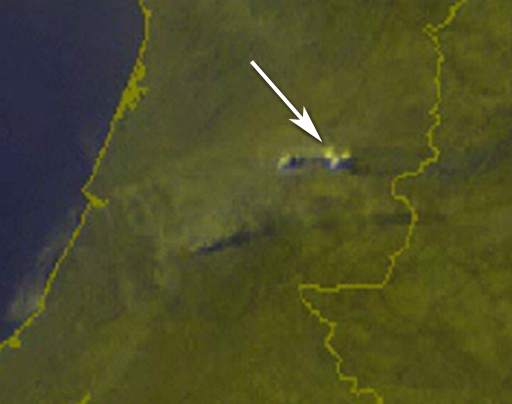
An example of Meteosat Second Generation. This RGB, which uses the HRVIS channel for red and green and IR10.8 for blue, shows a smoke cloud towards the center of the image and immediately northeast some pyrocumulus clouds (white arrow).

Figure 5.29 - Aerosol Index from the OMI (Ozone Monitoring Instrument) sensor onboard NASA's AURA-satellite on 25 August 2007 (during the forest fires in Greece). Source: Tropospheric Emission Monitoring Internet Service (TEMIS).

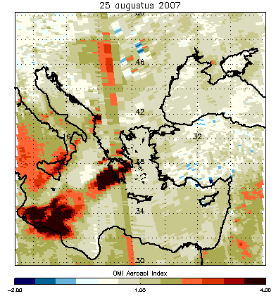
This image of the aerosol index measured by the OMI (Ozone Monitoring Instrument) instrument on 25 August 2007 clearly shows the soot of the fires blown from the Peloponnesus in Greece to Libya.

Figure 5.30 - Tropospheric NO₂ column density [1015 molecules/cm²]. Source: Tropospheric Emission Monitoring Internet Service (TEMIS). Click to enlarge.

NO₂ column density (in 1015 molecules/cm²) from the OMI (Ozone Monitoring Instrument) sensor onboard NASA's AURA-satellite from 23 to 26 August 2007 (during the forest fires in Greece). NO₂ (together with formaldehyde) is a gas released by burning biomass and was detected over Greece and also downwind, even in the coast of Libya.

Figure 5.31 - Formaldehyde concentration (in 1015 molecules/ cm²) from the SCIAMACHY sensor onboard the ESA satellite ENVISAT. 26 August 2007.

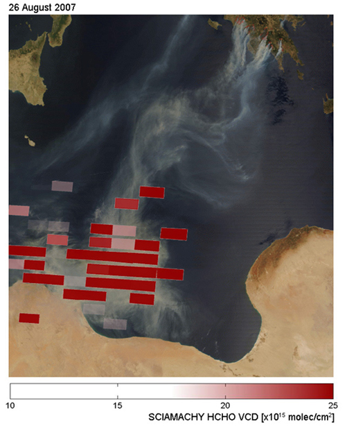
An example of formaldehyde concentration on 26 August 2007, derived from the SCIAMACHY sensor onboard ESA's ENVISAT satellite. Formaldehyde (together with NO₂) is a poisonous gas released by biomass burning and was detected off the coast of Libya. Note also that, again, the smoke in the background image has more contrast over sea than over land.

Did you know!

ash particles produced by fires have diameters in the range 2-20μm and that very intense fires can even generate giant ash particles with diameters up to 1 mm!?! Well ... it´s true and, in fact, the diameter of the particles influences their deposition velocity. For example, particles of 0.5μm diameter have a deposition velocity over water of around 0.003 cm/s and particles of 10-20μm diameter have a deposition velocity of around 10 cm/s.

Between 0.5 and 20μm (interval in which ash diameter fits), you may simply assume that the larger the particle the sooner it will get to the surface! But note that the deposition velocity also depends on other factors like wind speed, atmospheric stability and surface characteristics (Seinfeld and Pandis, 1998 and Reid et al, 2005).

One instrument you might not immediately think of for the purpose of monitoring forest fires is radar. However, experiences from the Portugese Meteorological Service have shown that it can be of use. In the example you see here (Figure 5.32), a Maximum Reflectivity (Max Z) radar image is showing two fires under a northerly flow in central Portugal on 20 August 2007. In this case, higher values of reflectivity are caused by ash particles and not by hydrometeors!

Fig 5.32 - Maximum Reflectivity (Max Z, in dBZ) from the Radar Coruche/Cruz do Leão in central Portugal on 20 August 2007 at 17:50 UTC (Source: Portuguese Met. Service, Remote Sensing Division).

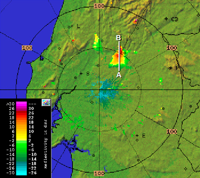
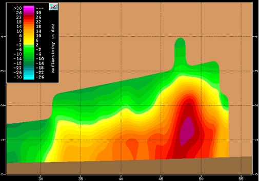
A cross section is retrieved in a north-south direction (see white line) as seen from the east. You can see how a stronger signal is found right from the surface up to around 4 km, in the location of the fire (Figure 5.33).

Fig 5.33 - Cross Section of Reflectivity (in dBZ) retrieved in a north-south direction as seen from the east (white line in Figure 5.31). Source: Portuguese Met. Service, Remote Sensing Division.

Aerosol Forecast

The MACC (Monitoring Atmospheric Composition & Climate) project computes forecasts of "anthropogenic aerosols", defined as organic matter, black carbon and sulfate aerosols that are emitted from fires and other, mostly anthropogenic, sources. An example of simulated aerosol optical depth (AOD), including emissions derived from the latest observed fire distribution and assimilation of space-borne AOD observations, including emissions derived from the latest observed fire distribution and assimilation of space-borne AOD observations, is shown in Figure 5.34. The fire distribution maps used as input in these simulations are obtained from the D-fire subproject, as mentioned in the Hot Spots Gallery subchapter.

Fig 5.34 - MACC forecast of total aerosols optical depth (AOD) at 550 nm for 16 October 2011 at 03:00 UTC. Click to enlarge.

The optical depth of the simulated resulting smoke aerosols (organic matter, black carbon, and sulphate) from the fires that occurred in Greece in August 2007 are presented in figure 5.35. The left panel shows the fire intensity observed by the SEVIRI instrument in terms of fire radiative power (FRP per unit area at 25 km resolution, reddish color bar) and the optical depth of the simulated resulting smoke aerosols (AOD, bluish color bar), for the 26 and 27 August. Images on the right show concurrent MODIS observations; the simulations and observations of the Greek fire plumes display very similar shapes.

Burnt Areas

In addition to fire hot spots and smoke, satellite sensors are also able to detect burnt areas. Check the true color RGB image (0.66 μm; 0.55 μm; 0.47 μm) in Figure 5.34 (click to enlarge and play the animation) for an area in northern Portugal at the beginning of June 2006 (Fig. 5.35 and Fig 5.36).

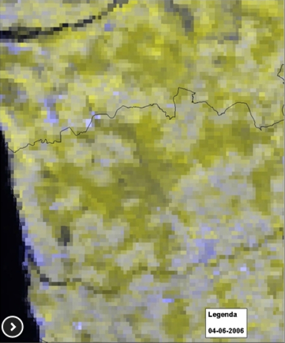
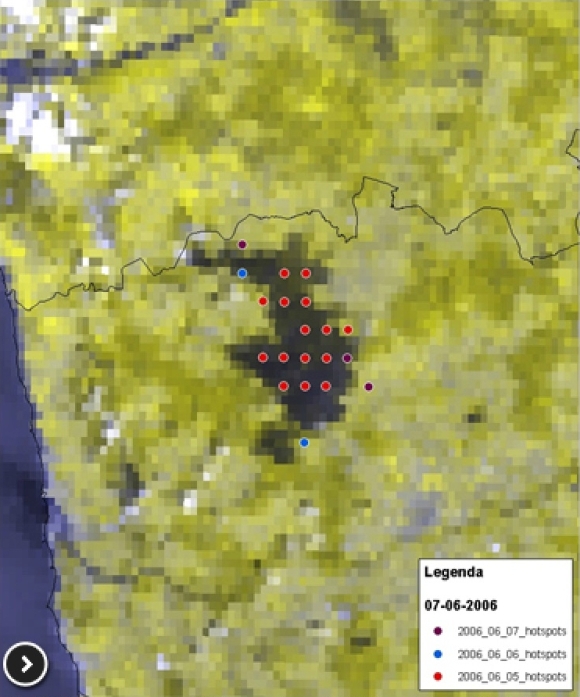
Fig 5.35 - True color RGB image from MODIS on 4 June 2006 before a series of forest fires and Fig 5.36 - True color RGB image from MODIS on 7 June 2006 after 3 days of forest fires over northern Portugal. Dots represent pixels where fires have been detected (hot spots): red on 5th, blue on 6th and purple on 7th June 2006 (Café and Tavares, 2008).

A change in the signature of the surface is clearly visible! The darker pixels correspond to a wide burnt area that resulted from several fires that took place over three days. The dots correspond to the hot spots (dots have different colors according to the day the fires occurred).

However, automatic detection of burnt areas is not straightforward. Did you know that warm burn scars from recent fires can be confused with cloud shadows in true color RGBs, like the one you see on the left in the image above?

In fact, aside from thresholds tests that depend on surface reflectivity, threshold tests with bands close to 3.9 μm and 10.8 μm may also be applied to distinguish cloud shadows from warm burn scars. For the warm burn scar (not an on-going fire!), the brightness temperature difference between these two bands [BT3.9 - BT10.8] is higher than for cloud shadows. Some scientists agreed on a threshold value of 6.5 K for this difference during experiments in Africa.

A burnt area product for the MODIS sensor has been in use since 2006 on a 500 metre spatial resolution. This product is based on an iterative algorithm with threshold tests. It uses bands 2 (841-876 nm), 5 (1230-1250 nm) and 7 (2105-2155 nm). Bands 2 and 5 are sensitive to burning and experience a decrease in reflectance after a fire. Band 7 is used as a reference since it changes less with burning.

For this MODIS product, threshold tests with bands 2, 5 and 7 may also not distinguish fire-affected areas from temporary changes. The changes may, in fact, be related not only to shadows, but also to undetected residual clouds or soil moisture changes. The MODIS burnt area algorithm uses a temporal constraint to solve this problem. Basically, it consists of tracking burnt area candidates on consecutive days and checking if an initial detection has future consistency.

Before we go and start to look at some examples of satellite images with burnt areas you have to keep in mind the following:

The burnt area algorithm for MODIS makes use of many more days of consecutive observations than the three days shown in this simplified exercise that you just took. And of course cloud shadows are more problematic with polar satellite observations than with 15 minute images from a geostationary platform!

Burnt Area Gallery

Next we will present you with some example cases form Europe on the detection of burnt areas using the MODIS satellite. The cases are from NASA's Earth Observatory website.

First, in the Côte d'Azur in France, there is a burnt area within the black rectangle.

Fig 5.36 - MODIS image on 28 July 2003 from NASA´s TERRA satellite.

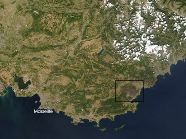
The brownish shade east of Marseille is due to the decreased albedo resulting from the fires.

Fig 5.37 - MODIS image on 28 July 2003 from NASA´s AQUA satellite.

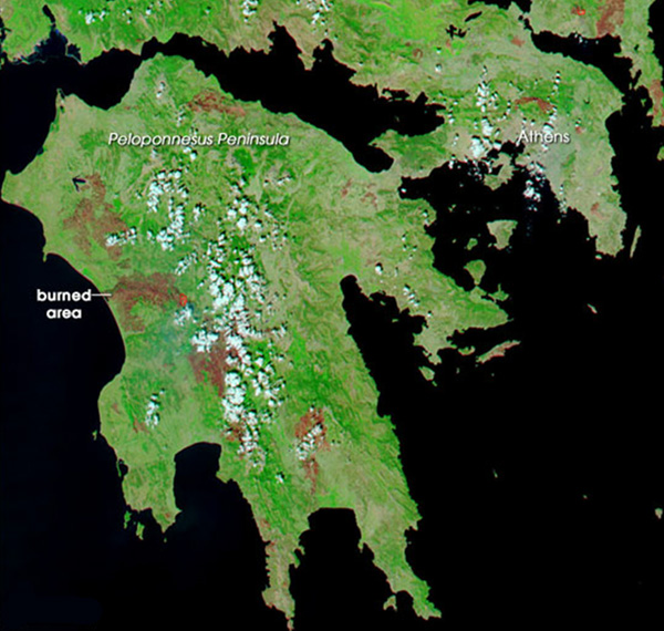
A slightly older example shows the aftermath of the fires that raged over Greece during the hot summer in 2003. Brownish areas depicting the burned regions can be identified all over the Peloponnesian Peninsula, as well as north of Athens. This MODIS RGB image with a 250 m spatial resolution is composed of a combination of visible and infrared bands (2.155 nm/876 nm/670 nm).

Fig 5.38 - MODIS image on 29 July 2008 from NASA´s TERRA satellite.

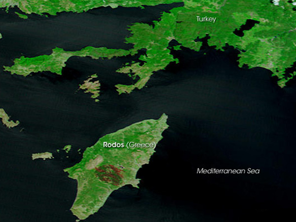
A shot of the island of Rhodes from the summer of 2008. The large burnt area in the middle of the island is easily recognizable.

The burnt areas show as brown in the colored image. This RGB image with a 250 m spatial resolution is composed of a combination of visible and infrared bands (2.155 nm/876 nm/670 nm).

Fig 5.39 - A map of burnt areas over Portugal between 1997 and 2004.

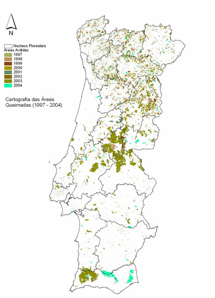
This map of Portugal was obtained with the AVHRR sensor onboard the NOAA satellites between 1997 and 2004, and it shows the burnt areas. Each color corresponds to a different year according to the color code in the top left corner of the image.

The summer of 2003 with its deadly heat wave and the effect it had on the wildfires in Portugal was already mentioned in the introduction of this training module. The severity of that summer's situation is clearly shown by all the brown color.

Did you know that fires may originate an albedo seasonal change?

Yes, scientists believe that fires in Africa may modify the natural vegetation cycle, which is usually driven by the precipitation regime related to the north-south migration of the Intertropical Convergence Zone [ITCZ].

The explanation lies in the following:

The albedo of open land is generally higher than forested land. Due to ITCZ migration, maximum albedo values are usually reached at the end of the dry season (April/May) and minimum albedo values are usually reached at the end of the wet season (October). In other words, this means that vegetation removal due to drought events originates an increase in the albedo. It is also well know that a high albedo value causes a radiative sink for the atmosphere near the surface, affecting the surface energy balance and suppressing moisture and precipitation.

On the other hand, fires originate surface darkening. In Africa, this darkening has been proved to increase the radiation absorption at the surface, excluding situations when smoke and aerosol are present in the atmosphere. Scientists believe that this increase of absorption at the surface is likely to strengthen convective activity. Therefore, it is considered that processes of albedo change due to fires should even be included in climate modelling for Africa.

Summary

This last chapter of the CAL module showed you how to detect and monitor forest fires using various remote sensing techniques.

Satellite images and their interpretation played a major role. The MSG satellites have shown us that the IR3.9 channel is suited for detecting forest fires. We looked at the reasons why this channel it suited for detecting hot spots (such as temperature responsivity and sub-pixel response). It is also possible to detect smaller scale phenomena such as smoke by combining this channel with the HRVIS. We also saw a range of high-resolution examples from the MODIS instruments onboard the TERRA and AQUA satellites, whichprovided a spectacular view of the fires.

We also found that products from the OMI (Ozone Monitoring Instrument) could reveal the presence of NO2 and formaldehyde in the smoke. A 2007 case study of Greece showed how this plume of smoke swirled over the Mediterranean and into Libya. Another second case study of Portugal showed that monitoring the smoke is also possible with meteorological radar.

The chapter closed with the difficulties of detecting burnt areas with both polar and geostationary satellites. The shadows of clouds are often mistakenly identified as burnt areas. Some examples from Modis concluded the chapter.

Limitations

However, you should be aware that some limitations on the remote detection of fires do exist. Sensors are limited by their resolution, and thus can only detect hot spots of sufficient size.

You should also note that not all hot spots are wild fires - volcanos and power plant explosions can reach the same temperatures as fires and can be confused with them. During the day, a reflection of the sun on a lake's surface may also look like a fire.

For smoke detection, the limitations are mainly over land, where there is a reduction of contrast.

The chapter closed with the difficulties of detecting burnt areas with both polar and geostationary satellites. The shadows of clouds are often mistakenly identified as burnt areas. All these limitations show us why algorithms that process all the information together are so important: they provide thebest information attainable through remote observation.