Chapter II: Xynthia's life cycle
Table of Contents
The early stages
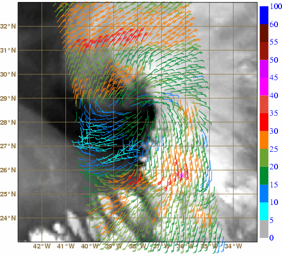
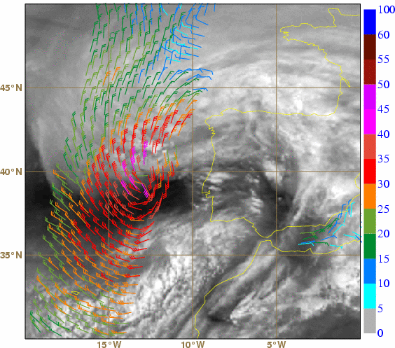
The low-pressure system that later become Xynthia was observed by ASCAT on 25th February 2010 between 12:52 and 12:55 UTC (Figure 2.1.1). The nearest (in time) MSG observation corresponds to the 12:45 UTC image (MSG scan time of this area around 12:55 UTC) and confirms how the two ASCAT swaths surround the most active area, as the dry intrusion and cloudy areas clearly lie between the two swaths. The left swath shows northeast winds ranging between 25 and 30 kt (Beaufort 6 to 7), corresponding to the northwest quadrant of the low. To the east of the most active area, winds in the right swath are in general below 20 kt.

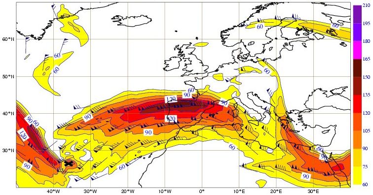
The low-pressure system formed in a subtropical area of the North Atlantic (at around 30°N and east of Bermuda) within a southwesterly flow at low and mid levels and within an upper level wave embedded in the westerly/zonal flow. The stratospheric air corresponding to the dark area in WV6.2 image (and between the ASCAT swaths) was bordered to the west by an intense northwest branch of the polar jet (Figure 2.1.2), which interacted with the already existing surface low.
This area had a sharp southeast-northwest temperature gradient between a warm moist tropical air mass and a colder and drier air mass (Figure 2.1.3), with strong dipoles of warm and cold advection in the low levels. In addition there was a strong upper-level positive vorticity advection east and northeast of the low centre (Figure 2.1.4) causing upward motion. Also, a strong vertical wind speed shear existed over the area. At this time, deep convection could already be seen on marked WV boundaries (Figure 2.1.1).

The low-pressure system was in a region where the sea surface temperature (SST) ranged between 20 and 23 °C south of 30°N and between 17 and 19 °C north of 30°N. Later on 25th, a second low coming from the lower latitudes was absorbed by the main low, yielding a complex low-pressure system, which remained over the SST gradient area until the middle of the following day, 26th February (Figure 2.1.5).
This first ASCAT observation of the system (25th around 12 UTC) may seem disappointing as it fails to find the centre of the low as well as the location of the wind maximum. However, ASCAT provides a hint of the asymmetry of wind speed at this stage (Figure 2.1.1), namely regarding the northwest (more intense) and southwest quadrants (less intense). And, of course, it is only the beginning of the story...
Xynthia is born
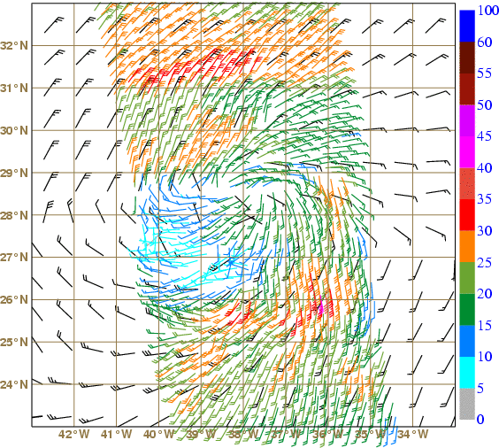
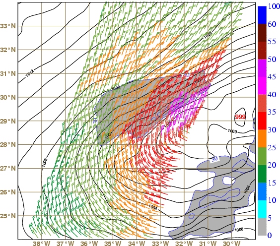
Around 00UTC on 26th February one of the ASCAT swaths passed right over the low-pressure system (Figure 2.2.1). At this time the main depression reached its most southerly position after moving approximately 1900 km southeastward in the last 24 hours. The pressure began to fall significantly after this time, as by now the low-pressure system was right below the left exit area of a jet streak (135/150 kt at 300 hPa) (Figure 2.2.2) and stratospheric air was reaching its lower level (~500 hPa).
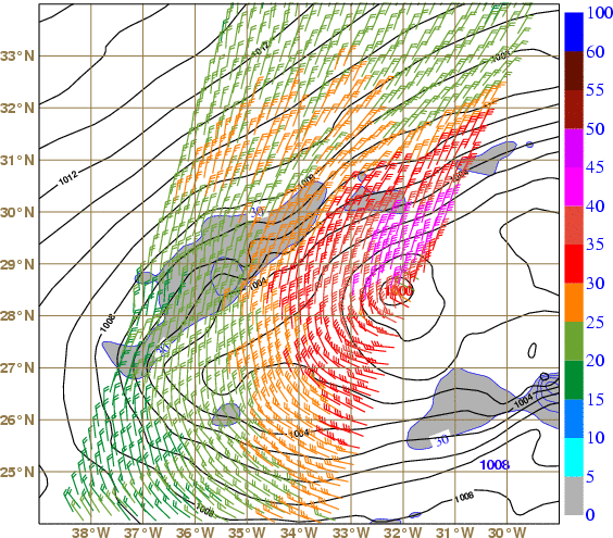
At this stage ASCAT measured winds in the 30-35 kt range to the north and south of the system (Figure 2.2.1), that is Beaufort 7 to 8 (near gale to gale). In fact, in the southeast border of the storm centre ASCAT wind was even reaching the 37.5-42.5 kt range (Beaufort 8 to 9, gale to strong gale). Taking into account these wind speed values, if this storm were to be considered of tropical nature, being below 30°N, it would already be reaching tropical storm intensity. The ECMWF wind analysis at 00:00 UTC was practically coincident with the ASCAT pass. Therefore, ASCAT data were likely to have been assimilated into this ECMWF model run. The ECMWF analysis reproduced winds reaching 30 kt on both the north and south areas referred above, but nevertheless missed the narrow region of strong gale winds (Figure 2.2.3, left).
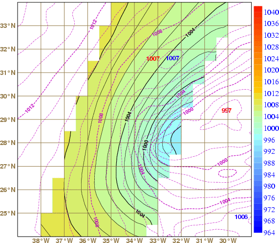
In fact, the minimum pressure centre at the surface was not totally clear in ECMWF's MSLP analysis, although a value of 1003 hPa, approximately at 27.5°N 37°W was proposed (Figure 2.2.3, right). In Figure 2.2.3, the MSLP analysis is overlaid with the surface pressure derived from ASCAT winds, which is obtained with the Planetary Boundary Layer Model from the University of Washington (UWPBL, more details in Patoux et al, 2003). This promising estimate, which is valid both in mid-latitudes and tropics, suggests a minimum of 1004.3 hPa, therefore very close to the ECMWF estimate, but around 150 km to the northwest, at 28.5°N 38°W. These estimates correspond closely with a 00:00 UTC observation of 1003.4 hPa from a drift buoy located around 26°N 38°W, where the ECMWF and UWPBL estimates are around 1005 hPa and 1005.5 hPa, respectively.

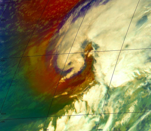
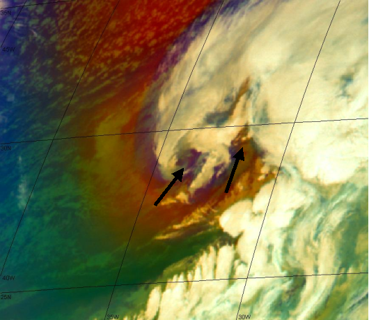
It was during the 26th that this low-pressure system was named Xynthia. Between 04:00 and 08:30 UTC Xynthia was surrounded by dry stratospheric air, depicted by brown-reddish shades in the Airmass RGB image from MSG (Figure 2.2.4). Between 05:00 and 06:30 UTC it was possible to detect what seems to be an eye in the centre of the low (Figure 2.2.4, left). In the following hours, two new particular regions of stratospheric (dry) air intrusion became very clear in the images (depicted by black arrows in Figure 2.2.4, right). At this early stage (until around noon the same day) Xynthia had incipient frontal characteristics at mid and upper levels, although there was already a ridge of potential equivalent temperature at 850 hPa with large gradients (mainly meridional) over the area (Figure 2.2.5). In the tongue of warm air, convection was very active and organized. In the course of the day Xynthia's frontal structures became better defined.
Fast-moving Xynthia starts to deepen
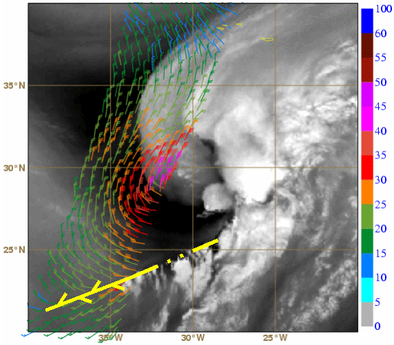
Around noon on the 26th, when passing south of the Azores, the storm was still showing much convective activity, with a prominent cloud head as well as an impressive dry intrusion. Although at this stage ASCAT only observed the western flank of the storm, it measured strong gale winds (Beaufort 9) up to 45 kt and, in a larger area, over 40 kt, thus still inside the reliable range for ASCAT winds (Figure 2.3.1). To the south a clear wind convergence line was found in the ASCAT wind product (depicted in yellow in Figure 2.3.1). It connects with a line of convection in WV6.2 (depicted as an instability line, also in yellow), but unfortunately the ASCAT winds do not reach this area. This line matched the sharp air mass gradient area that existed for the past 24 hours around the Tropic of Cancer (see Figure 2.1.4).
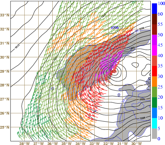
In the ECMWF model, the wind speed threshold of 45 kt was clearly reached by the analysis and the 12 hours forecast, but not by the 24 and 36 hours forecasts where maximum wind speed were in the 35-40 kt range (Figure 2.3.2). Regarding the area of higher wind speeds, naturally the analysis field fits the ASCAT observations better (check how grey shades cover red, brown or magenta wind barbs). Minor discrepancies in the border of the 30 kt threshold area may be attributed to the 30 minutes time difference between ASCAT pass and analysis instants, as the depression has moved northeastward very rapidly, at a mean speed of around 35 kt during the previous 6 hours and 80 kt (!) in the following 6 hours, according to ECMWF analysis. This would amount to a difference of 1/3 to 2/3 of a degree of longitude in just half an hour!
Regarding forecasts, both the 12 and 24 hours forecast missed the intensity of wind speeds in Xynthia southwestern quadrant. The 36 hours forecast shifted the highest wind speeds almost 2 degrees of longitude to the west, well above the expected shift due to the non-coincident ASCAT pass time.
 |
 |
 |
 |
Regarding the pressure field, the ECMWF MSLP analysis field on 26/02/2010 at 12:00 UTC showed a large low-pressure system, with two sub-lows but with the absolute minimum value (997 hPa) in the northeastern sub-low, around 29.5°N 30°W (Figure 2.3.2). This pattern was also suggested by the 24 hour forecast, but not by the 12 and 36 hours forecasts, which identified a main low-pressure system on the west side. At 12:00 UTC a drift buoy located close to the southwestern sub-low, at 28.5°N 32.5°W, reported 994.4 hPa, around 5 hPa deeper than ECMWF analysis for that location.
ECMWF analysis suggested a drop of 7 hPa in 6 hours, between 12:00 and 18:00 UTC. A constant pressure drop in this period would result in a decrease of ~0.6 hPa every 30 minutes. As the ASCAT surveyed the area slightly after 12:30 UTC, it could be acceptable to apply a pressure drop of 1 hPa to the ECMWF analysis and buoy values mentioned above. This would result in a MSLP of 996 and 993.4 hPa for the analysis and buoy, respectively, at the time of the ASCAT pass.
The UWPBL model output (using ASCAT wind as input) clearly depicts the curved isobars on the west side of the storm, most likely the southwestern sub-low (Figure 2.3.3). The minimum sea level pressure along the pass was 995.4 hPa at 28°N 32°W, therefore lying between the "time-corrected" values derived from the ECMWF analysis and buoy observation. Note, however, that neither ASCAT nor buoy caught Xynthia's centre.
At this time Xynthia still had its vertical trough axis slightly leaning west, although at higher levels the ECMWF analysis showed only an emerging wave embedded in the western flow. As mentioned, the frontal nature became clearer from model fields but was still better depicted in lower levels than in mid and higher levels (Figure 2.3.4). Xynthia continued its northeasterly path as a deep low with strong winds at all levels, always embedded in a very humid and warm air mass, with regions of intense warm advection (Figure 2.3.5). Based on subjective analysis, it is safe to say that Xynthia still remained a complex low for the following 24 hours, until it reached the Portuguese coast.

Xynthia as a bomb
Around 22 UTC on the 26th, ASCAT passed once more over Xynthia, while pressure in the centre was dropping intensively. With a pressure decrease in the last 24 hours of 14 hPa at 18:00 UTC on the 26th and 18 hPa at 00:00 UTC on the 27th (ECMWF analysis), Xynthia could, at this stage, be classified as an explosive cyclogenesis, or bomb (Figure 2.4.1).
From the point of view of ASCAT, this was an interesting pass for two main reasons:
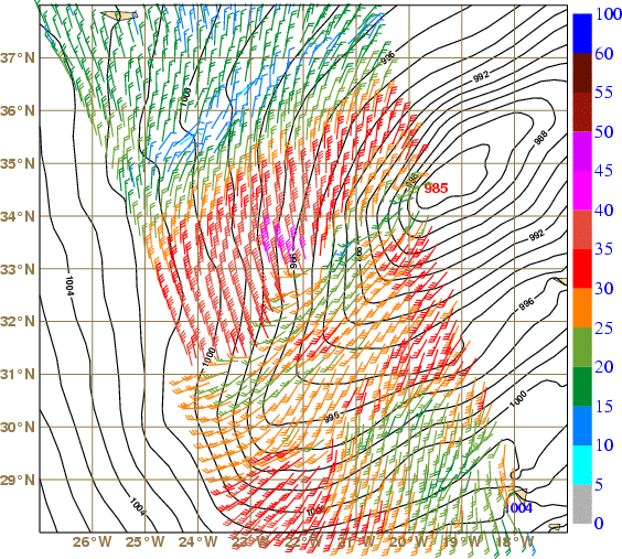
i) ASCAT clearly showed a well defined boundary between southwesterly and northwesterly winds, in the leftmost part of the swath, suggesting a cold front wind pattern at the surface (as plotted in Figure 2.4.2, left). Nearer to the centre of the swath, opposite winds (northeasterly and southwesterly) could be found along an axis from 33°N 22°W to 34.5°N 20°W, suggesting the existence of more than one low. Finally, in the rightmost part of the swath, the wind pattern fit to the existence of a warm front. In general, the north side of the storm presented higher wind speeds (in the range 40-42.5 kt) than the south side where winds did not exceed 35 kt. ASCAT thus suggested that Xynthia was still a complex low at the surface (see two possible lows in Figure 2.4.2, left).
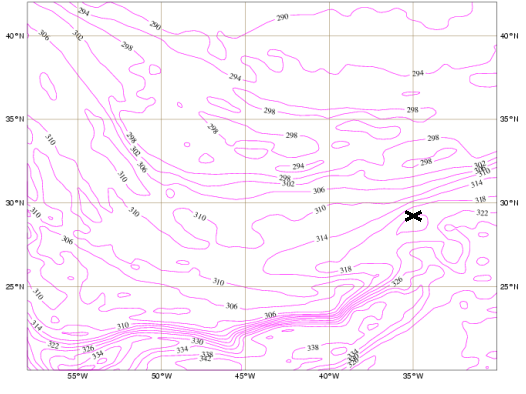
Using only buoy observations in the area, the minimum pressure at 22:00 UTC would be located near 34°N 20°W, on the right edge of the ASCAT swath, with an estimated value of 984 hPa (see black cross in Figure 2.4.2, left).

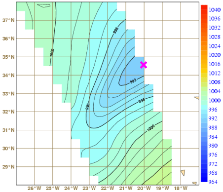
A minimum of 991.1 hPa could be found at 34.5°N 20°W from the UWPBL derived surface pressure (Figure 2.4.2, right), which puts it half a degree to the north of the "buoy estimate". However, this represented an overestimation of around 7 hPa, which would be consistent with an underestimation of the wind speed by ASCAT.
In the attempt to determine the centre, the "buoy estimate" and the "ASCAT estimates" (from both wind and surface pressure patterns) were not a perfect fit. However, there were clear benefits to using ASCAT patterns of both wind and surface pressure. Regarding wind speed and minimum pressure values, data from both buoy and ship were still used for "real-time tuning".
ii) the instant of the ASCAT pass differed from both the ECMWF model analysis and forecast times - by around 110 and 70 minutes, respectively (Figure 2.4.3). This was not negligible at this phase as the storm was still moving very fast northeastwards (averaging around 40 kt (!) between 18:00 and 00:00 UTC). In this case, a mismatch in the overlay of forecast and ASCAT winds (speed and/or direction) cannot be taken too seriously, because with such a velocity, differences of up to around 1.5 degrees in longitude could be expected even if forecast and ASCAT were exact matches (not to mention changes related to the pressure drop). However, the 9-h forecast indicates a secondary low to the southwest of the main low, in accordance with ASCAT. This feature was not captured by the following ECMWF analysis (on the 27th at 00:00 UTC), but as mentioned this analysis was almost 2 hours after the ASCAT pass.

In this period, Airmass RGB images made it possible to distinguish some cold air patches (in darker blue) among clouds and stratospheric air intrusions near the low centre (Figure 2.4.4). Several cloud layers with their corresponding movements are also plotted in Figure 2.4.4, as suggested by the sequence of images between 18:00 and 21:00 UTC (Figure 2.4.5).
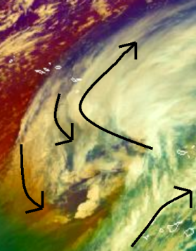
Figure 2.4.5 - MSG Airmass RGB between 18:00 and 21:00 on 26/02/2010. Click the image to enlarge and start the animation.
Xynthia passed northwest of the Madeira Islands overnight as a deep storm. Surface observations from the Madeira archipelago recorded high wind gusts, reaching 145 km/h (78.4 kt) at the mountain station of Areeiro (1590m) at 23:30 UTC on 26th, and an hourly precipitation maximum of 15.6 mm between 03:00 and 04:00 UTC on the 27th (and 56.2 mm in 6 hours, between 00:00 and 06:00 UTC). However, these precipitation amounts are not totally unusual in the mountains of Madeira, and therefore not as high as one might expect, taking into consideration the air mass involved, the direction of flow and the topography of the main island. In a way, Xynhtia was starting to reveal itself to be more a wind storm rather than a precipitation storm.
ECMWF analysis suggested 985 hPa at 34°N 19°W at 00:00 UTC on the 27th (Figure 2.4.6) and a drift buoy reported 986 hPa around 37°N 16°W which suggests another minimum further northeast. The model outputs show Xynthia with well defined frontal characteristics (note how the Thermal Front Parameter exceeds the colour-coded scale in Figure 2.4.6) related to strong temperature advections both on the warm and cold sides. The frontal patterns from the model analysis do not disagree with the subjetive analysis based exclusively on ASCAT winds (Figure 2.4.2).
Approaching shore
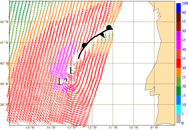
During the 27th, Xynthia started to approach the European continent. Around 10:30 UTC, ASCAT located Xynthia off the west coast of Portugal (Figure 2.5.1, top left), with maximum wind speeds in the 40-45 kt range (basically strong gale wind or Beaufort 9). As before, identifying the storm centre was difficult from MSG satellite images alone. The HRV RGB at 10:00 UTC (Figure 2.5.1 top right) indicated that the centre of the storm was defined by warm low clouds (in light yellow), with the convective clouds with colder tops (in white bluish) only located in the north quadrant of the storm. This suggested again that Xynthia was still essentially a windstorm at the time and no longer a storm mainly associated with convective episodes. Using surface observations at 10:00 and 11:00 UTC (SYNOP, ship and buoy) along with MSG images one could conclude that only one centre existed, with a possible minimum of 970 hPa or even lower around 39°N 12.5°W (at 10:00 UTC) and 40°N 12°W (at 11:00 UTC) - see Figure 2.5.1, bottom. At 11:45 UTC the yellowish low clouds in the HRV RGB image defined a clear curl pattern, in what may have been one of the best representations of Xynthia's centre from MSG observations at this stage.
 |
 |
 |
 |
Looking in detail into the ASCAT wind pattern and surface pressure estimate from UWPBL (Figures 2.5.2 and 2.5.3), some additional interesting features emerge:
- The pressure minimum of 985 hPa by ASCAT/UWPBL suggests a clear overestimation by this algorithm, when comparing to the minimum pressure estimated through surface observations around 970 hPa (ECMWF MSLP 9h forecast for 09:00 UTC indicated 971 hPa at approximately 38°N 14°W and in the 12:00 UTC analysis it reached a minimum of 973 hPa). This overestimation by ASCAT/UWPBL can be either related to the boundary model characteristics or to a possible underestimation of wind speed by ASCAT. This may suggest the real wind to be stronger than Beaufort 9. Remember though that ASCAT still has a reliable range up to 50 kt (Beaufort 10), excluding wind speeds corresponding to Beaufort 11 and 12.
- Apart from the main pressure centre already mentioned, a second pressure minimum appears around 41.5°N 11.5°W (also 985 hPa), on the eastern edge of the plotted ASCAT swath. This may indicate either the existence of a secondary low, or simply a wave along the warm front that is carrying an airmass northwards ahead of Xynthia on its northeasterly trajectory.
- Around 39°N 13.5°W, opposing winds can be found in a pattern that, again, suggests the existence of a third centre. In this case, the overall northwesterly flow around the opposing winds may support the idea that the ambiguity removal scheme on ASCAT wind processing (see Chapter 1.2 for more details) may have not made the best choice in this case.

So far Xynthia (in its complex structure) had been moving "alone" over North Atlantic with two large surface ridges, one to the northwest and another to the northeast, isolating the storm. Throughout the 27th Xynthia, without losing its identity, entered into a larger complex low-pressure area to the north, the main centre of which was located west of the British Isles.
Also at this stage the role of upper levels seemed to be decisive, as dry stratospheric intrusions and the jet stream had a clear influence on Xynthia's dynamics. Accordingly, high values of vorticity advection and temperature advection at 300 hPa were found, as been happening since the 25th. At 06:00 UTC on the 27th, the upper geopotential disturbance caught up with the lower disturbance (still just a wave in the main large scale upper trough) so that the previous tilt upstream was lost. In the following hours they would still be in phase, but Xynthia would continue to deepen until 00:00 UTC on the 28th.
The Bay of Biscay and a large storm surge
12 hours after passing the west coast of Portugal, ASCAT captured Xynthia once again, this time over the Bay of Biscay (Figure 2.6.1). In the meanwhile, the centre of Xynthia passed around 150 km off the coast of Portugal during the afternoon of the 27th, producing a 91 km/h (49.2 kt) wind gust in the coastal station of Viana do Castelo at 15:20 UTC. Xynthia already had caused 1 casualty due to a falling tree in a village in northern Portugal around 14:15 UTC. In the rest of country, greenhouses and electrical grids were damaged by strong gusts, with power outages lasting until the next day. Also, around 1000 occurrences of floods and landslides demonstrated that Xynthia was not only a windstorm after all.
During the afternoon Xynthia may have made a slight landfall in Spain, passing along Fisterra and Islas Sisargas, with the METAR observation from La Coruña showing a minimum of 969 hPa between 16:30 and 17:30 UTC. Near the coast, gusts peaked 98 km/h (53 kt) in La Coruña at 16:30 UTC and 100 km/h (54.1 kt) in Vigo at 15:30 UTC, with stronger gusts inland as high as 167 km/h (90.3 kt) throughout the day. Three casualties occurred in Spanish territory as a consequence.

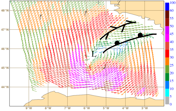
At 21:00 UTC Xynthia was again over the sea, with subjective surface analysis from available surface observations (SYNOP, SHIP and BUOY) suggesting a centre around 45°N 5°W with an MSLP value of 970 hPa or lower. However, the elongated shape of the MSLP field analysis over the Bay of Biscay, with a small trough stretching east-northeastwards, could suggest either the possibility of two centres or a frontal trough.
Around 21:50 UTC, the ASCAT wind pattern supported the possibility of a frontal trough, as it was consistent with a warm front located east-northeast of a dominating low around 45.5°N 5.5°W (Figure 2.6.2). ASCAT also clearly showed that there were now stronger wind speeds along Xynthia's southern border, with storm winds of 52.5-55 kt (Beaufort 10) at 44°N 5°W, that is, only 50 km off the Asturian coast (but outside the usually accepted reliable range for ASCAT). The ASCAT wind directions were consistent with BUOY/SHIP observations (in black barbs in Figure 2.6.2, obtained within 10 minutes of the ASCAT pass) but wind speeds were generally 5 kt weaker in ASCAT.
As a reference, the maximum wind speed was about 55 kt for the closest ECMWF forecast (around 1 hour before) and about 60 kt for the closest ECMWF analysis (around 2 hours later), both in the south quadrant of the storm. However, the time difference between these values and those from the ASCAT pass is too large for a straightforward comparison. This is especially true taking into account Xynthia's displacement speed of 30 kt over the area, which could lead to discrepancies of up to 1 degree in latitude even for a perfect fit between model and reality. Nevertheless, it should be stressed that the ECMWF model placed and defined Xynthia's intensity with a reasonable accuracy over the Bay of Biscay since the run on the 25th at 00:00 UTC. The forecasted location was even closer to its real location after the run on the 26th at 12:00 UTC (that is, by the time of the third ASCAT pass analyzed in this study (see chapter 2.3)), which was when Xynthia started to deepen.
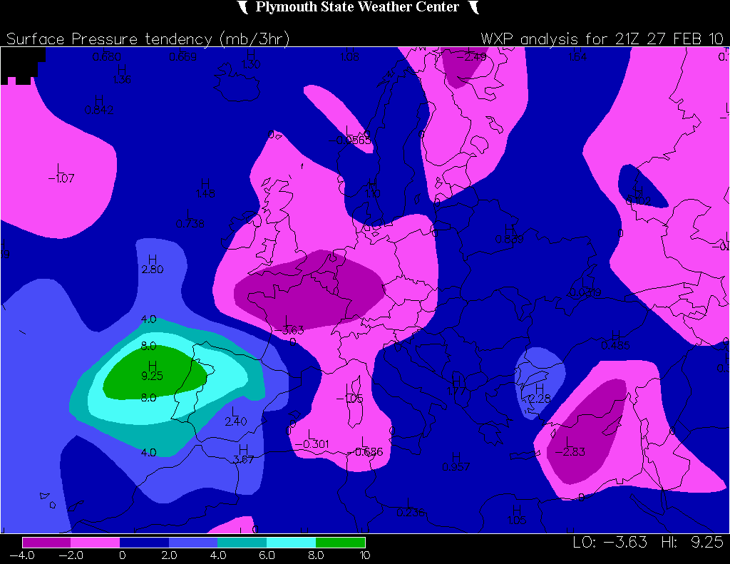
Since its genesis, Xynthia has shown an almost permanent surface pressure tendency dipole along its trajectory. In fact, not only did pressure drop very quickly but it also rose very quickly behind the storm. This could be seen very clearly at 21:00 UTC on the 27th (Figure 2.6.3). In its northeast trajectory across the Bay of Biscay, Xynthia's centre passed slightly to the north of the buoy located at 42.5°N 5°W, which had a minimum surface pressure of 969.4 hPa at 23:00 UTC and an intense pressure rise of 10 hPa in the following hour (Figure 2.6.4).
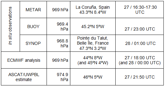
Xynthia, already in an occlusion phase, made landfall again, this time near Belle Île in France between 01:00 and 02:00 UTC on the 28th (see observations from the weather station Pointe du Talut in Figure 2.6.5). Table 2.6.1 summarizes the minimum MSLP values for this stage of Xynthia.
The pressure drop over the Bay of Biscay produced a strong storm surge on the coasts of Spain and France. An example of such a storm surge was depicted by MOG2D model output, which suggested a maximum sea level rise of 85 cm (Figure 2.6.6). In fact, the tide gauge of La Rochelle (Charente-Maritime Department) in France recorded a tide height of 8.01 m that corresponded to a storm surge of 1.53 m, resulting both from low surface pressure and high wind speeds. This storm surge height was not only the highest ever recorded since the instrument was installed in 1997, but was also higher than any height recorded in the Brest tide gauge (also on the French coast) in 150 years. The storm surge produced an extreme and vast flooding event in the coastal areas of the Charente-Maritime and Vendée Departments, which resulted in at least 53 casualties in France alone.
Xynthia filling up in the North Sea
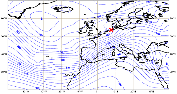
After landfall in France, the storm moved along the coastlines of Belgium, the Netherlands and Germany. Xynthia was now weakening, with a mean sea level pressure of 976 hPa at 18:00 UTC on the 28th over the Dutch/German border according to ECMWF analysis (Figure 2.7.1). Since its genesis, Xynthia was characterized by an upper level wave rather than a sharp trough. However, a short through could be detected in the upper levels at 18:00 UTC on the 28th (Figure 2.7.2).

The ASCAT view of Xynthia over the North Sea in the late afternoon on the 28th was basically a glimpse of the northwestern part of the storm (Figure 2.7.3). In fact, the closest MSG IR10.8 image (at 19:45 UTC) and in-situ wind observations (at 20:00 UTC, see Figure 2.7.4) are better tools for identifying the centre location at that time, when it was already close to the German/Danish border.
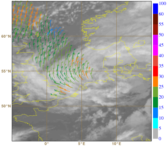
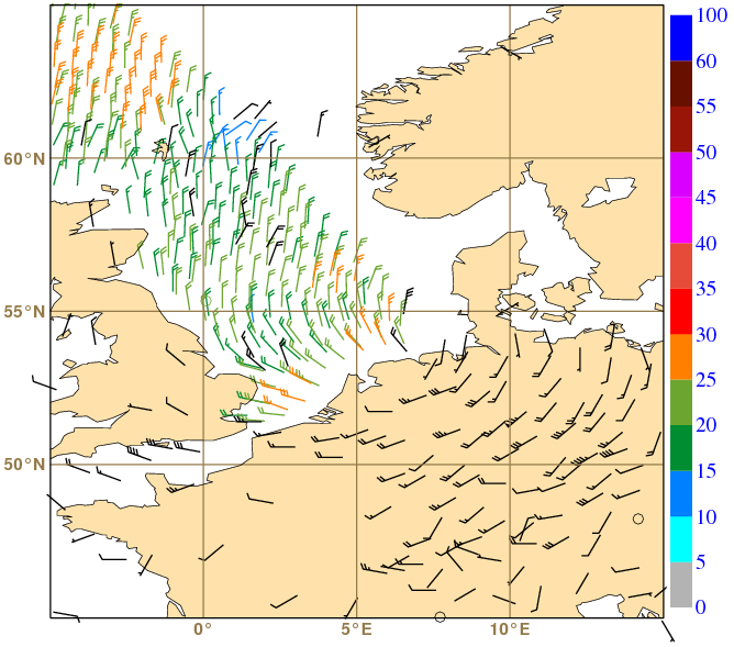
Although ASCAT wind speeds were now below the 30 kt threshold over the North Sea (Beaufort 6 to 7), the storm still presented strong and damaging winds in the south quadrant - see for example a 75 kt (~140 km/h) mean wind report in a SYNOP observation at 20:00 UTC in Figure 2.7.4. At this time Xynthia became associated with one casualty in Belgium and four in Germany, as well as with electricity and aviation disruptions in the affected regions.
The Baltic Sea and the end of Xynthia
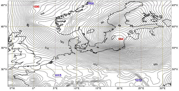
By the time it reached the Baltic Sea, Xynthia was no longer a cause for alarm for local forecasters. ASCAT did not depict the depression centre clearly, but nevertheless it depicted the wind patterns in Xynthia's southeast quadrant, with wind speeds below the 30 kt threshold (Figures 2.8.1 and 2.8.2).
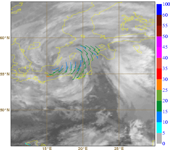

ECMWF forecasts after 25th February were all indicating a low-pressure system over the Baltic Sea area at this time. Remember that by the 25th the precursor disturbance that later become Xynthia was already present over a subtropical area of the North Atlantic and could be assimilated by the models. After the 25th, the minimum sea level pressure forecasts for the depression at 9:00 UTC on 1st March ranged from 978 to 988 hPa (10 hPa spread), depending on the run, while the surface observations suggested a minimum pressure of 982 hPa at that time. According to the forecasts since the 25th, three countries could have reclaimed the location of the low at this instant, as it changed in a box with 5° longitude and 2.5° latitude:
- Near Gdansk in the north coast of Poland (105 hour step, run 25th 00:00 UTC);
- South of Malmö, Sweden (93&81 hour steps, run 25th 12:00 UTC and 26th 00:00 UTC);
- Between the south of Sweden and Ronne island, Denmark (69, 57 and 45 hour steps, runs 26th 12:00 UTC and 27th 00:00 and 12:00 UTC);
- Close to Öland Island, Sweden (33, 21 and 9 hour steps, runs 28th at 00:00 and 12:00 UTC and 1st March at 00:00 UTC).
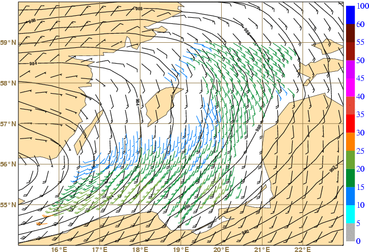
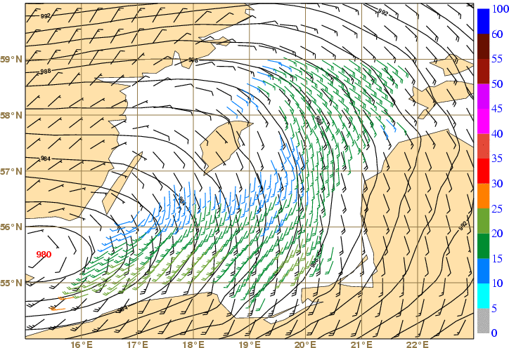
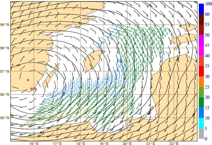
The superposition of ASCAT winds with forecasts at 09:00 UTC from the last four 00:00 UTC runs is shown in Figure 2.8.3 and depicts how the ECMWF model tuned Xynthia's centre location on consecutive runs, with slight eastward or northeastward shifts every day.
 |
 |
 |
 |
After the run on the 28th 00:00 UTC (33 hour step, lower left in Figure 2.8.3) the low centre remains over coastal Sweden, close to Öland Island. The location in the 9 hour step (lower right in Figure 2.8.3) fits best not only to surface observations, but also to the ASCAT wind pattern around 9:40 UTC, 40 minutes after the forecast time.
At 12:00 UTC on 1st March, Xynthia was still near the Swedish islands of Öland and Gotland also with 982 hPa in its centre (ECMWF analysis). During this day Xynthia slowed down, with an easterly displacement of 15-20 kt, which was clearly below the speed it had attained before. Despite its occlusion stage, there was still a warm sector, bringing milder air to these regions ahead of the storm. At 18:00 UTC Xynthia was located between Gotland Island and Estonia (Figure 2.8.4) and it continued its path towards the Gulf of Riga, making its last landfall late that day. Thereafter, Xynthia weakened in the northwestern part of Russia and, according to the University of Berlin (which named the storm in the first place!), made its last appearance on the weather charts on 5th March 2010.