The Xynthia Storm by ASCAT

Introduction

This case study will cover Xynthia, a storm that developed and evolved over the North Atlantic in late February 2010. Its progress was tracked by the ASCAT sensor onboard the EUMETSAT METOP-A satellite. First, a summary of Xynthia's development and impact is presented in Chapter 1.1 and a short description of ASCAT winds is presented in Chapter 1.2. Chapter 2 focuses on various ASCAT observations of Xynthia, covering several phases of its life cycle. Throughout the whole case study you will be able to enlarge the images by clicking on them. If there are multiple images, hovering the cursor near the edge of the image will reveal a button that allows you to toggle between images. Chapter 3 includes a summary of the case study.

The Storm

Xynthia had its genesis on 26^th February and its life cycle lasted for eight days. Its genesis was related to an already existing low-pressure system that formed on 25^th February east of Bermuda over a subtropical area of the North Atlantic (Figure 1.1.1).

Figure 1.1.1 - Geopotential (black lines in gdam), temperature (red lines in °C) and wind barbs at 500 hPa. Analysis from the ECMWF model for 25/02/2010 at 12:00 UTC. The black cross in the lower left corner represents the surface low with a MSLP of 1006 hPa that later became Xynthia.

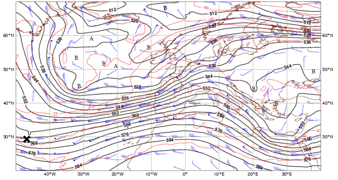
This region was characterized by warm and moist air at low levels and an upper level wave embedded in the westerlies. Xynthia's path was quite unusual, crossing the Atlantic from subtropical latitudes towards Russia. In its early stage over subtropical latitudes, Xynthia showed organized deep convection that was quite well depicted by satellite imagery. Later Xynthia lost its convection activity, mainly after passing the west coast of Portugal (Figure 1.1.2).

Figure 1.1.2 - MSG Airmass RGB between 21:00 on 25/02/2010 and 00:00 UTC on 02/03/2010. This animation follows the centre of the storm during the whole trajectory.

Xynthia had an explosive development and a rapid displacement between the 26^th and 28^th, bringing a strong flow of warm air over all continental Europe until its end on 5 March. At the surface, Xynthia was mainly a complex low until its landfall in the early hours of the 28^th on the French Atlantic coast. At the upper levels it was rather difficult to detect its related short-wave trough, which was embedded in a large-amplitude upper trough for most of its life cycle.

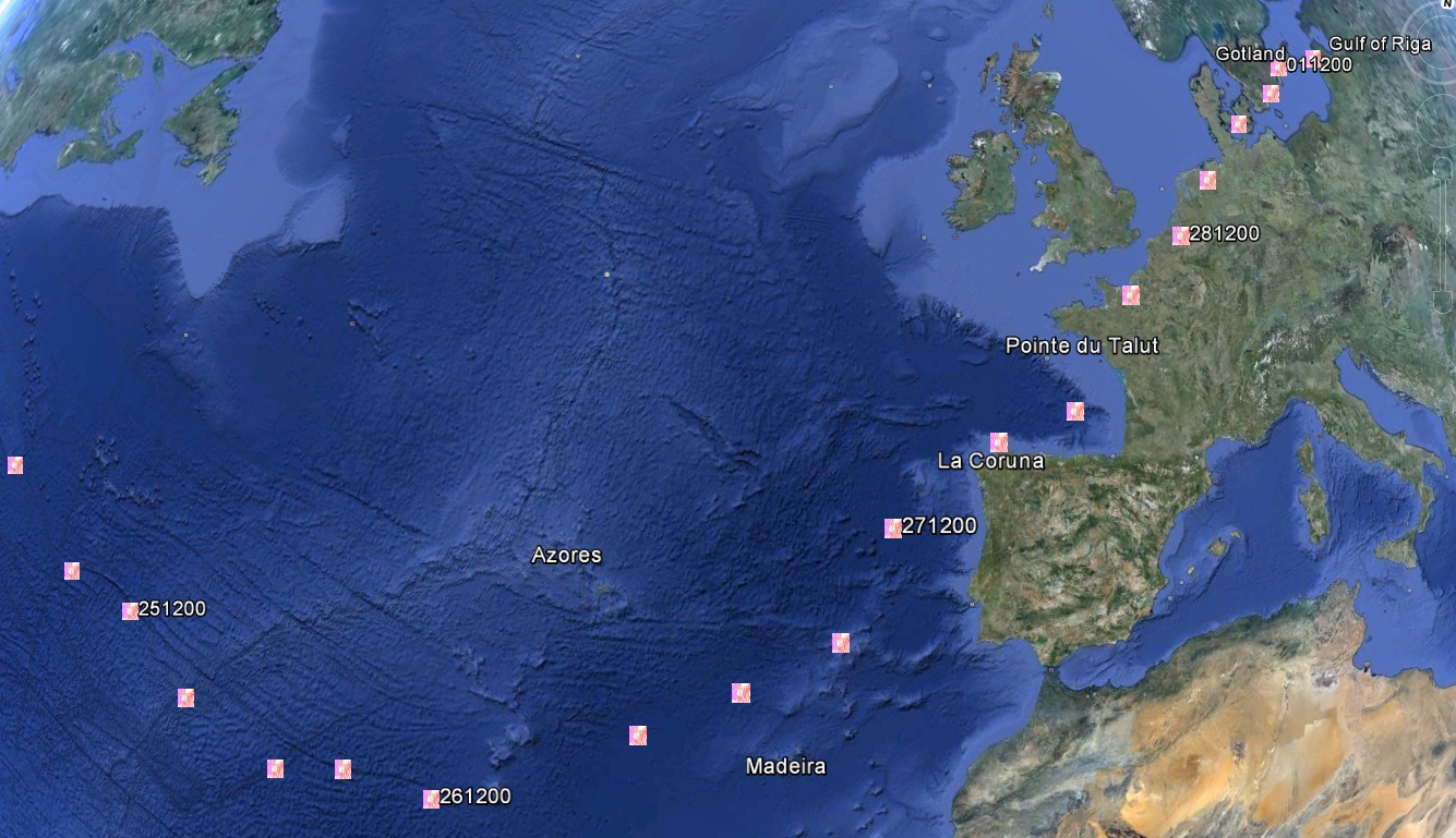
The severe storm was mainly a windstorm with reports of damaging winds from the Madeira Islands to northern Europe, with gusts exceeding 150 km/h (81 kt) in some regions. This large spatial coverage over the European territory was another distinctive aspect of Xynthia, as can be seen in Figure 1.1.3. There were also reports of large amounts of precipitation (both rain and snow) but these were not as unusual as the wind observations. In western Europe and mainly in France, Xynthia caused around 60 casualties, which resulted from drownings caused by severe storm surge events. Also, the storm caused significant damage and destruction, with trees being uprooted, roofs untiled and electrical grids being seriously affected, cutting off power in over a million households in France and Portugal. Total economic losses caused by Xynthia were estimated at € 3.6 billion in all the affected countries.

Figure 1.1.3 - Xynthia's trajectory between 25^th February 2010 at 00:00 UTC and 1^st March 2010 at 18:00 UTC according to 6 hourly ECMWF model analysis. The date/time is plotted every 24 hours after 25^th February at 12:00 UTC. Google Image.

The ASCAT sensor

ASCAT stands for Advanced SCATterometer. It is a microwave radar instrument onboard the EUMETSAT polar orbit METOP satellites, and it estimates wind (speed and direction) over the ocean, retrieves soil moisture and identifies snow and ice.

Scatterometers are active radar instruments and therefore both emit and receive microwave radiation. This radiation has the advantage of not being affected by clouds and this is why scatterometers are known to be able to scan the surface in almost all weather conditions. With regard to wavelength, there are in fact two types of scatterometers: C band (such as ASCAT) and Ku band (such as OSCAT, the scatterometer onboard the polar orbit Indian Space Research Organization OceanSat2 satellite, not used in this case study). Note, however, that for Ku band scatterometers (therefore not ASCAT) the backscatter can be affected by intense rainfall, so data from these areas is less trustworthy.

ASCAT is composed of two sets of three antennas that cover two distinct areas located to the left (one set) and to the right (the other set) of the satellite track, therefore being considered a double swath scatterometer (Figure 1.2.1), unlike Quikscat or OSCAT, which are single swath scatterometers.

Figure 1.2.1 - ASCAT geometry (Source COMET/EUMETSAT).

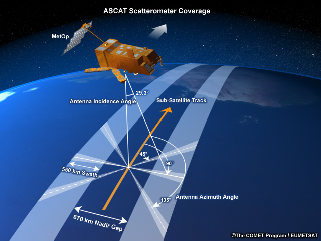
The three antennas on each side correspond to three different angles (azimuth angles). For instance, for the set of antennas facing to the right, the azimuth angles are 45° (fore beam), 90° (mid beam) and 135° (aft beam). This results, as the METOP satellite moves forward at 7 km/s, in three backscatter measurements for the same area, the so-called sigma-naught triplets.

In the nadir gap (area with no ASCAT data), scatterometer measurements would lack sensitivity to wind speed and/or wind direction and therefore are not effective. Nadir wind speed (no direction) is obtained by satellite radar altimeters that emit a radar pulse to the nadir (incidence angle of 0°). For ASCAT, incidence angles vary between 25° and 65°, yielding two swaths 550 km wide with a gap of 670 km between them.

ASCAT emits microwave radiation with a wavelength of 5.7 cm. This radiation is resonant with centimeter-scale ocean waves of comparable wavelength due to the so-called Bragg scattering mechanism, and is sent back to the sensor. This backscatter radiation coming from the water surface can then be processed in order to compute near-surface ocean wind speed and direction.

This capability relies on the assumption that the small-scale ocean waves responsible for the backscatter are in equilibrium with the wind. As wind speed increases, surface roughness also increases and more microwave radiation is scattered towards the direction of the radar source (Figure 1.2.2).

Figure 1.2.2 - Schematic representation of microwave scattering and reflection at a smooth (a), slightly rough (b), and rough (c) ocean surface. Retrieved from Stoffelen (1998). Since the cm-scale ocean roughness is aligned with wind direction, the radar backscatter depends on the the pointing direction of the radar beam with respect to the wind direction. As such, the radar backscatter depends on both wind speed and wind direction, i.e., on the wind vector.

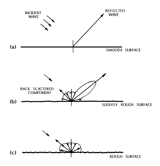
As a reference it can be stated that Bragg scattering dominates for incidence angles between 25 and 80°, which clearly covers the range of incidence angles for ASCAT.

The wind retrieval algorithm relies on the observation of the same ocean area from different perspectives (different azimuth and incidence angles). The core of the algorithm is composed by a Geophysical Model Function, which relates the triplets of backscatter (sigma-naught) with wind speed and direction (Verhoef et al, 2008, Stoffelen, 2009). The wind retrieval algorithm generally yields two wind directions, from which a final solution is obtained using an ambiguity removal procedure based on the use of NWP forecast data and spatial pattern analysis.

Before using ASCAT winds users should still consider the following:

• In this case-study, ASCAT winds correspond to the 12.5 km sampling interval (the finest so far), which showed better verification results than the 25 km sampling interval product.
• ASCAT winds are 25-km areal winds and are practically instantaneous. Therefore, strictly speaking, ASCAT winds cannot be directly compared to buoy wind speeds, which are local (in-situ observations) and correspond to a 10 minute time period. Also, ASCAT cannot be directly compared to the NWP global model's 10m winds, which may miss small-scale details.
• ASCAT winds are in fact equivalent-neutral winds (that is, winds that would occur in neutral stability atmospheric conditions and are only a function of the wind stress on the ocean surface). Equivalent-neutral winds may be easily converted to and compared to real buoy and NWP winds. As a global mean, equivalent-neutral winds are +0.2 m/s (+0.4 kt) higher than real 10-m winds, but this difference obviously depends on the local atmospheric stability conditions. Note that ASCAT winds better correspond to equivalent-neutral winds, since scatterometers, rather than responding to the real 10-m wind, do respond to sea surface roughness (see more details in Portabella and Stoffelen, 2008).
• The reliable range for ASCAT wind speed is 0-25 m/s (0-50 kt), with a standard deviation of 1 m/s (2 kt) and a correlation of 0.95. ASCAT winds somewhat underestimate wind speeds above 20 m/s (by 2-3% percent), and an enhanced calibration is forthcoming. Please be aware of this fact in operational forecasting activities, such as when comparing ASCAT winds to model outputs for any particular case (see more details in OSISAF).
• Regarding wind direction, note that ambiguity removal errors may occur. These may be identified by areas where the wind direction is opposed (i.e., is 180 degrees wrong). These errors do not occur often, but unfortunately happen particularly in dynamically active regions where the ECMWF model's first guess has large positional errors in fronts and/or lows.