Chapter IV: Physical Background Of Lee Waves
Table of Contents
- Chapter IV: Physical Background Of Lee Waves
- Trapped And Vertically Propagating Lee Waves
- Rotor Clouds
- Breaking Waves
- The Brunt-Väisälä Frequency
- The Scorer Parameter
- The Wave Length
- The Froude Number
- Exercises
Lee Waves
Lee waves are characterized by a periodic change of pressure, temperature and height of an idealized air parcel in an atmospheric air current. Lee waves were discovered in 1933 by German glider pilots. Glider pilots use the upwind area of lee waves to gain height. Other parts of lee clouds such as rotor clouds present a considerable threat for aircraft (areas with severe turbulence). In meteorology a difference is made between two major types of lee waves: trapped lee waves and vertically propagating lee waves.
Trapped And Vertically Propagating Lee Waves
Trapped lee waves have horizontal wavelengths of 5 - 35 km. They are trapped in a layer with high static stability and moderate wind speeds, usually in the lowest 1-5 km of the troposphere. Trapped waves occur when wind speed above the mountain increases sharply with height and when stability decreases in the layer just above the mountain top. As the wave energy is trapped within the stable layer, these waves can propagate far downwind of the mountain crest. The image below shows a schematic of trapped lee waves.

Figure 1: Schematic of clouds related to trapped lee waves. © COMET Program
For vertically propagating waves, the wave energy propagates in the vertically and not horizontally as with trapped waves. They occur when static stability increases above the mountain peak and when the wind speed does not increase significantly with height. They typically extend vertically up to the higher troposphere and are tilted backwards with height towards the mountain chain (figure 2). Due to their greater vertical extension, the wave energy dissipates more rapidly downstream compared to trapped lee waves, which leads to a smaller overall horizontal extension of the wave pattern. Vertically propagating waves are often accompanied by strong downslope winds (e.g. Foehn and Bora) especially when there is a "cloud gap" visible between the mountain chain and the first lee clouds.
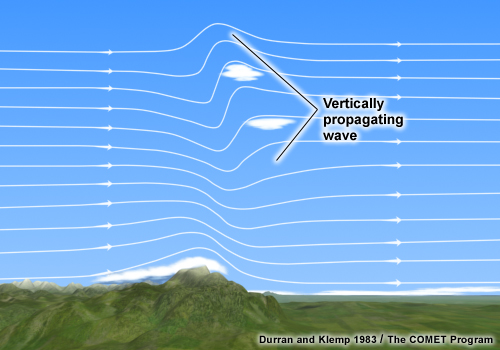
Figure 2: Schematic of clouds related to vertically propagating lee waves. © COMET Program
The Day Microphysical RGB below (figure 3) shows trapped lee waves over southern France, Sardinia and Tunisia (whitish-blue), and vertically propagating lee waves over the Alps (orange-red). While the former consist of water drops, the latter are composed of small ice crystals in higher atmospheric levels. As the ice crystals do not sublimate in the wave trough once they are formed, they remain visible as a homogenous shield of small ice crystals.
Figure 3: Day Microphysical RGB (MSG) from 21 January, 2005 at 12:00 UTC.
Rotor Clouds
Rotor clouds form at lowest levels and are a form of lee eddy. The air in the cloud rotates around an axis parallel to the mountain range. These clouds are associated with severe turbulence and strong vertical motions. At the bottom of the rotor cloud the wind direction is opposite to the gradient wind. Rotor clouds, filmed in fast motion, show a kind of "waterfall" effect (see the video below). Rotor clouds belong to the group of lenticularis clouds.
Figure 4: Rotor clouds over the Colorado Front Range. Credits Steve Zimmermann
Updrafts and downdrafts on both sides of the rotor cloud can exhibit wind speeds comparable to the background flow. The heaviest turbulence usually occurs near the first rotor cloud after the mountain crest. The height of the rotor cloud can exceed the mountain top by more than 1000 meters. Observations show that turbulence is more severe when the first rotor cloud forms further downstream of the mountain crest.
Figure 5: Schematic of a rotor cloud (WMO, 1978)
Breaking Waves
Breaking waves can be observed when vertical wind shear (also directional shear) exceeds a critical value. Wave slopes get steeper and steeper with increasing vertical shear until the top of the wave overruns the lower part (similar to breaking waves of the sea). Subsequently the laminar flow turns into a turbulent flow, inverting the preexisting stable stratification by mixing cold air with warmer air below. Breaking waves are found in both the lower atmospheric levels and in the jet level with negative wind shear below the tropopause (see chapter 5b).
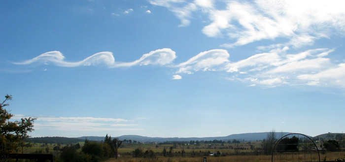
Figure 6: Breaking waves over Mount Duval in Australia. ©GRAHAMUK, CC BY-SA 3.0
The more stable the atmosphere, the higher the wind shear can be before waves start to break. This also means that a less stable atmosphere favors turbulence in a region with lee waves.
The Brunt-Väisälä Frequency
The Brunt-Väisälä frequency N [s-1] describes the oscillation frequency of an air parcel in a stable atmosphere.
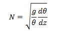
where θ is the potential temperature in [K], g the gravitational acceleration in [m/s2] and z the height in [m].

Figure 7: Buoyancy oscillation with advection. © The COMET Program
In a stable air mass, a vertically perturbed air parcel (e.g. by vertical lift in a mountain range) will have the tendency to come back to its initial position because the air parcel cools when lifted and warms up compared to the surrounding air temperature when dragged down. In this case, N2 > 0 and the oscillation frequency is given by N. In an unstable air mass, N2 < 0 and the vertically perturbed air parcel will move away from its original position instead of returning to it (e.g. convection).
The Scorer Parameter
The Scorer parameter l [m-1] is used to describe whether gravity waves will develop or not. It combines the Brunt-Väisälä frequency with characteristics of the vertical wind profile and is given by the following equation:
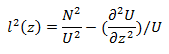
where N = N(z) is the Brunt-Väisälä frequency and U = U(z) is the vertical profile of the horizontal wind. Both quantities are determined from an atmospheric sounding upstream of the barrier. The first term on the right-hand side usually dominates.
The typical profile of the Scorer parameter shows a high gradient in low levels due to increasing wind speeds. When l2(z) decreases strongly with height, conditions are favorable for trapped lee waves. This is especially true if the decrease of the Scorer parameter occurs suddenly in the mid-troposphere, dividing the troposphere into two regions, a lower layer with large values (high stability) and an upper layer with small values of the Scorer parameter (low stability). At higher levels the Scorer parameter often shows values of about 0.5/km, rarely exceeding 1/km.
However, when l2(z) is nearly constant with height, conditions are favorable for vertically propagating mountain waves.
In the third case, when l2(z) increases with height, the conditions are not favorable for the development of gravity waves.
Note:
In practice, the Scorer parameter is derived from vertical sounding profiles of wind and temperature upstream of a mountain chain to forecast the probability of trapped lee wave development. In cases where the wind data has high vertical resolution, the second term on the right-hand side of the above equation (velocity-profile curvature term) can show values of similar magnitude as the first term. This again leads to a noisy profile of the Scorer parameter. Therefore, either the wind profile is smoothed before calculating the Scorer parameter or the second term is omitted. This is acceptable since Richard S. Scorer postulated an undisturbed air flow upstream of the mountain chain as prerequisite for his parameter.
The Wave Length
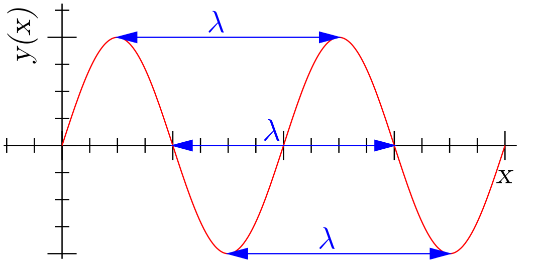
Figure 8: Plot of a sine wave showing three pairs of corresponding points between which wavelength (λ) can be measured. ©Richard F. Lyon, CC BY-SA 3.0
Wave length is the distance between two points with same phase (figure 8). The wave length of lee clouds depends on atmospheric stability and wind speed but not on topography. Short wave lengths occur in very stable atmospheric conditions with low wind speeds while high wind speeds and a less stable atmosphere generate longer wave lengths. The relationship between wave length λ [m], wind and stability is given by:

with l(z) being the Scorer parameter. Typically wave lengths are in the order of 5 to 35 km with an average around 10 km. Hence lee waves can be observed easily with today's geostationary satellite image resolutions as long as their wave length does not fall below 5 km in mid-latitudes.
In cases with complex orography (e.g. several mountain chains in parallel), lee waves may be damped or enhanced depending on the relationship between wave length and distance between the mountain chains (figure 9).

Figure 9: Schematic describing the interaction between wave length and complex topography (WMO, 1978).
The Froude Number
The Froude number establishes a relation between wind speed and atmospheric stability.
When an air stream hits an obstacle like a mountain chain, it has the possibility to either flow over it without being decelerated or to split and circle around both sides of the obstacle with the formation of an upstream decelerated area which propagates continuously upstream over time. The flow behavior depends largely on atmospheric stability and wind speed. The Froude number (here in the non-classical form) describes this behavior:

where U is the mean wind speed [m/s], H is the height of the barrier [m] relative to the height of the air stream and N the Brunt-Väisälä frequency [s-1]. When the Froude number Fr >> 1, the air tends to stream over the mountain chain, and in the opposite case (Fr << 1) it tends to contour the obstacle.
In the lower levels the wind needs more kinetic energy to crest the mountain than in levels slightly below the mountain top. Lower winds are therefore either blocked or deflected around the barrier, while higher up winds tend to pass over the mountain peaks. Typically, the wind will pass over the smallest elevations which in turn leads to a channeling effect as can be observed at many mountain passes in the Alps.
Figure 10: Airstream overflowing or bypassing a mountain.
Exercises
True or False
Select the correct statements:
The correct answers are: b), e), f)
Choose the right answer