Tutorial on Satellite Derived Wind Products

The Kinematic Extrapolation Method

The kinematic extrapolation of frontal cloud bands was one of the earliest applications of satellite-derived cloud motion vectors (CMV). This means that CMV were used to linearly extrapolate the displacement of a front in a time frame up to 2 hours (Very Short Range Forecasting - VSRF), assuming that the frontal cloud band continues its propagation invariably, i.e. in the same direction and with same speed as the CMV indicate.

Figure 16 shows the IR-CMV superimposed on a frontal system over Western Europe. It shows the displacement of the cold front (central France) towards the east, the displacement of the warm front (Switzerland and northern Italy) towards the southeast and parts of the occlusion (northern France, Belgium) towards the northeast.

Notice that since wind speed increases with height, the CMV are largest for high reaching clouds and small for low-level clouds. Due to the applied cross-correlation method, the CMV are not zero over bare ground or very low cloud fields like fog and low stratus (e.g. southeast Germany). This effect results from the selection of a 32 by 32 pixel search area which may contain different types of clouds (e.g. high and low clouds). Therefore this method works best with homogenous and high reaching clouds.

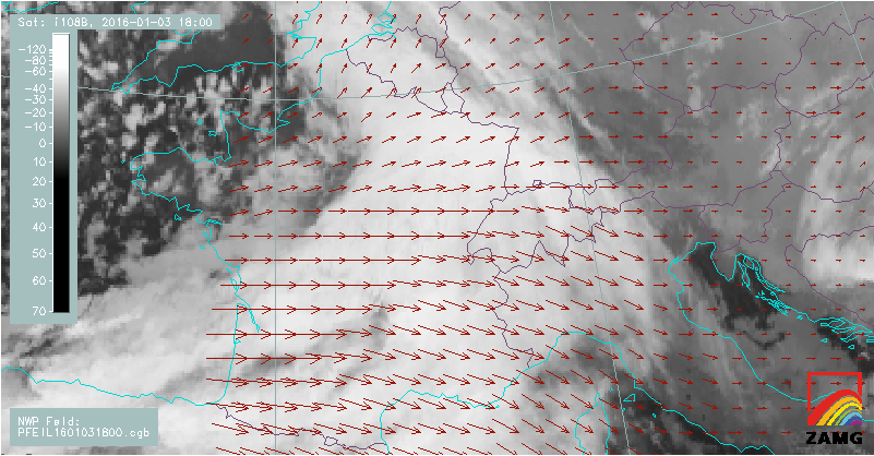
Figure 16: CMV derived from IR10.8 μm superimposed on a frontal system over Western Europe. The length of the red vectors is proportional to the displacement. The MSG image dates from 3 January 2016 at 18:00 UTC.

In the cold season, frontal systems are generally better suited for kinematic extrapolation than in the warm season because they show less dynamic changes. Figure 17 shows a visualization of the kinematic extrapolation method of the same frontal system as above applied to MSG 10.8 μm brightness temperatures (BT).

To better illustrate the frontal displacement, brightness temperatures are divided into classes and coloured accordingly:

Yellow: -30°C to -40°C

Red: -40°C to -50°C

Green: -50°C to -60°C

The corresponding lines in yellow, red and green indicate the position of the frontal system one hour later in time. The position of the lines is deduced with help of the CMV.

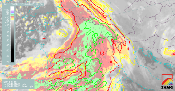
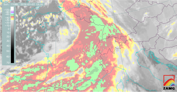
Figure 17: Kinematic extrapolation applied to cloud top temperatures. The MSG IR10.8 μm BT image dates from 3 January 2016, 18:00 and 19:00 UTC. Apply the slider to compare predicted and real cloud position.

It is of equal importance for the forecaster to know not only at what time the frontal system will arrive, but also when related weather phenomena like rain or snowfall will set in at a given geographical position. For this reason, kinematic extrapolation has not been applied to both clouds and synoptic reports of rain, drizzle and snowfall as shown in Figure 18.

As not all parts of the frontal system are connected to precipitation, the forecaster's attention is drawn only to the areas where precipitation occurs.

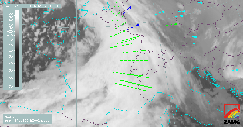
Figure 18: Rain (green), drizzle (blue) and snow (cyan) reports from synoptic stations linearly extrapolated 2 hours into the future (3 January 2016, 18:00 UTC to 20:00 UTC).

Note:

Kinematic extrapolation is a very simple method to forecast the propagation of cloud features and related meteorological phenomena in the domain of VSRF. A time step longer than 2 hours is rarely applicable for extrapolation due to dynamic changes within the frontal cloud band (e.g. embedded convection). Neither does this method account for orographic obstacles.

Verifying NWP Wind Fields With ASCAT Wind Data

ASCAT wind data provide detailed information on 10 meter surface winds over oceans and lakes. These wind vectors are far more precise than surface wind charts from model data as can be seen in Figure 19. Scatterometer winds show convergence and shear, areas with increased wind speed, the position of surface pressure minima and even the intensity of fronts near the ocean surface. Wind drag on the ocean surface induces waves which propagate and finally reach coasts. They can cause damage and life threatening situations for people living near the shore. High Swell also has a damaging potential for coastal areas but cannot be detected by scatterometers.

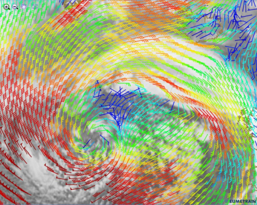
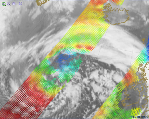
Figure 19: Model 10m wind speed (ECMWF) and ASCAT wind speed data from 5 January 2014 at 12:00 UTC. Apply the slider to compare predicted and real wind direction.

Figure 19 shows a comparison of NWP data with ASCAT wind speed data at 10 meters above the ocean surface for the storm Christina. While both data sources show good agreement, the scatterometer data has a much finer resolution and shows some discrepancies in the region of light wind speeds north of the pressure minimum (blue arrows).

By comparing measurements of wind speed and direction with NWP surface pressure fields, the meteorologist can evaluate the quality of the model forecast. Figure 20 shows such a comparison between ASCAT wind data and the ECMWF mean sea level pressure field. Taking a time delay of 2 hours between both fields into account, the position of the forecasted surface low is in good accordance with the measured data.

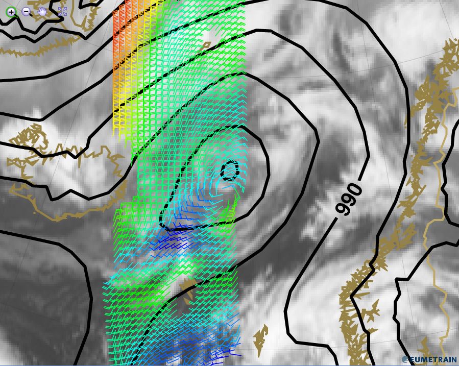
Figure 20: ASCAT wind field and ECMWF forecast (+12h) of the mean sea level pressure for 5 January 2014 at 00:00 UTC.

ASCAT wind data can be used to analyze the position and severity of surface fronts over the oceans. Figure 21 shows the cyclone Ruth, located west of the British Isles on 7 January 2014. At that time, Ruth had become a winter storm with gale force winds up to 8 Beaufort. ASCAT measured storm force winds, force 10 (50kts)! The ASCAT overpass shows high wind speeds near the center of the low (red wind barbs) and a steep gradient next to the Irish coast at the location of the yellow wind barbs.

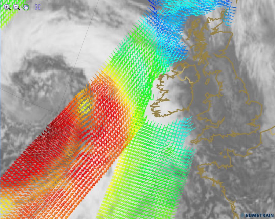
Figure 21: Two ASCAT overpasses over the storm Ruth on 7 February 2014 at 10:16 UTC (right stripe) and 12:01 UTC (left stripe). The IR10.8 μm image is from 12:00 UTC.

Within the next 12 hours, the southern part of Ireland and Cornwall were hit by the storm as it reached a force of 11 to 12 Beaufort. Valentia (Ireland) recorded 24 mm of rain in 24 hours.

The ASCAT measurements show strong surface winds over the Atlantic between Iceland and Greenland on 7 February 2014 at 12:00 UTC (see Figure 22). Strong surface winds transfer their momentum into the water and create waves. There is a high degree of correlation between wind speed and significant wave height.

Where ASCAT measurements show wind speeds between 35 and 40 m/s, significant wave height determined from Jason-2 reaches 7 meters and more.

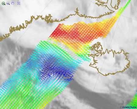
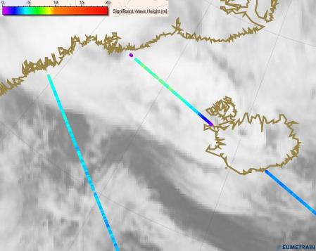
Figure 22: Comparison between ASCAT wind data and JASON-2 significant wave height data for 7 February 2014 at 12:00 UTC. Apply the slider to compare both data sources.

Upper Tropospheric Convergence And Divergence

This chapter deals with the EUMETSAT MPEF product "Divergence". The divergence is directly calculated from the field of Atmospheric Motion Vectors (Figure 23). Only high level vectors (above 400 hPa) are considered, and the horizontal resolution for the search area for the cross correlation method is 32 by 32 pixels. AMV are derived by tracking cloud and humidity features in the 6.2 μm WV channel. The MPEF Divergence product represents an atmospheric layer between 100-400 hPa rather than a specific atmospheric level.

EUMETSAT started to operationally disseminate the MPEF Divergence product in 2008 via EumetCast.

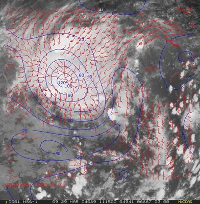
Figure 23: Atmospheric motion vectors derived from MSG 6.2 μm channel (red wind barbs) and divergence (blue lines) calculated from the AMV. The MSG IR10.8 μm image dates from 29 March 2009 at 11:15 UTC.

In this chapter, the AMV-based Divergence product will be presented as an additional tool for diagnosing upper-level environments favorable for deep convection. Although this product also covers tropical areas (e.g. Figure 8 over central Africa), we will concentrate on the mid-latitudes.

The MPEF Divergence product at mid-latitudes

At mid-latitudes, values of the MPEF Divergence product are much smaller than in tropical regions. The reasons for this are the weaker updraft of convective systems at mid-latitudes compared to tropical areas and the lower horizontal resolution of MSG images, which tends to smooth out information.

Upper-level divergence constitutes a favorable environment for deep convection. Acting together with low-level forcing mechanisms such as instability and moisture convergence, it provides an additional trigger for the development of deep convection.

Upper-level divergence is most often encountered at the north-eastern part of an upper-level trough (see Figure 24). If a frontal system is present this would be near the occlusion point and the left exit region of the jet streak.

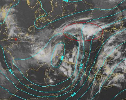
Figure 24: IR image from 22 April 2008 at 06:00 UTC with isolines of the geopotential height at 300 hPa. The red line indicates the area of divergent flow.

C. Georgiev and P. Santourette (2010) investigated 1166 deep convective cells and their position within a region of divergence in the MPEF Divergence product. Their results showed that 76% of deep convective cells initiated in areas of upper-level divergence indicated by the MPEF product.

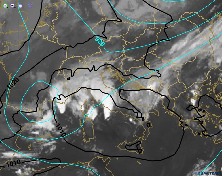
Example: 15 June 2014, 06:00 UTC

A weak surface pressure minimum is located over Italy and the surrounding Mediterranean Sea. The upper atmosphere is characterized by two upper-level troughs, of which only the stronger one over southern France can be seen in the isolines of the geopotential height at 300 hPa. The smaller upper-level trough located over Greece is only visible in the streamline field (see Figure 25).

Convective developments are present in the zone of divergent flow near both upper-level troughs (red circles).

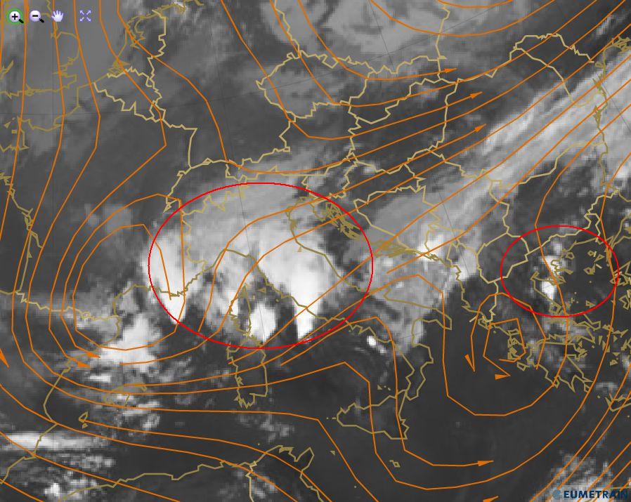Figure 25: IR10.8 μm image from 15 June 2014 at 06:00 UTC. 300 hPa geopotential height (cyan), mean sea level pressure (black), and streamlines at 300 hPa (brown). The red circles indicate the area of divergent flow at 300 hPa.

The MPEF Divergence product calculated from WV6.2 μm images indicates upper-level divergence in both regions. The light blue area in Figure 26 over the Mediterranean Sea south of France as well as the green area over Greece are in good agreement with the diffluent streamlines from the model forecast field. Convection had already developed in these areas 6 hours earlier.

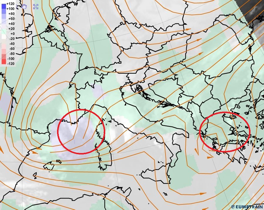
Figure 26: MPEF divergence product and ECMWF streamlines at 300 hPa for 15 June 2014 at 06:00 UTC.

The global instability index product (GII), which shows the lifted index (Figure 27), indicates strong instability in the affected regions. Upper-level divergence acts in favor of the development of deep convection.

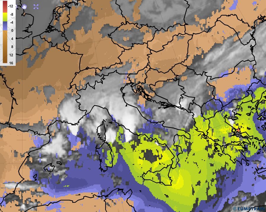
Figure 27: Global instability index (GII) for 15 June 2014 at 06:00 UTC.

Note:

Upper-level divergence alone is not sufficient to initiate the development of thunderstorms. But if it is present, it acts as a trigger in combination with other factors such as instability, orography and moisture convergence in lower levels to build a favourable environment for convective development. Upper-level divergence constitutes an effective trigger in the higher troposphere.