Chapter III: Snow RGB
Table of Contents
The main aim of this RGB type is to discriminate snow covered land from fog or low water clouds. Although several RGB types are usable for snow detection and for discriminating between snow and low clouds, it is the Snow RGB which provides the highest colour contrast between snow and water clouds (red-orange against white). This RGB type was tuned especially for this purpose.
Fog frequently forms over cloud-free snow surfaces in wintertime high pressures. Identifying foggy areas is important, for example because of traffic security. The Snow RGB is a daytime RGB.
The Snow RGB is composed of the reflectivity images calculated from the VIS0.8, NIR1.6 and the 3.9 micrometer channel (IR3.9).
Physical basis
Daytime snow detection
Snow RGB consists of three images: the snow is bright in one and dark in two components, while the water clouds are bright in all three components. This is the key of snow-water cloud discrimination and will ensure good colour contrast between the two.
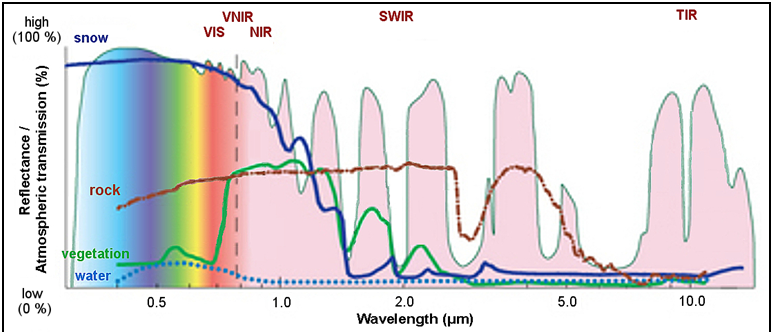
Fig. 1 shows typical reflectivity spectra of surface types. The snow reflectivity (blue curve) is high around 0.8 micrometer and low around 1.6 and 3.9 micrometers. The reflectivity of water clouds (not shown in Fig. 1) is high in all three channels.
| Figure 1: Reflectivity spectra of different surfaces. (Credit: Andreas Kaab, University of Oslo.) |
|
Water and ice cloud discrimination
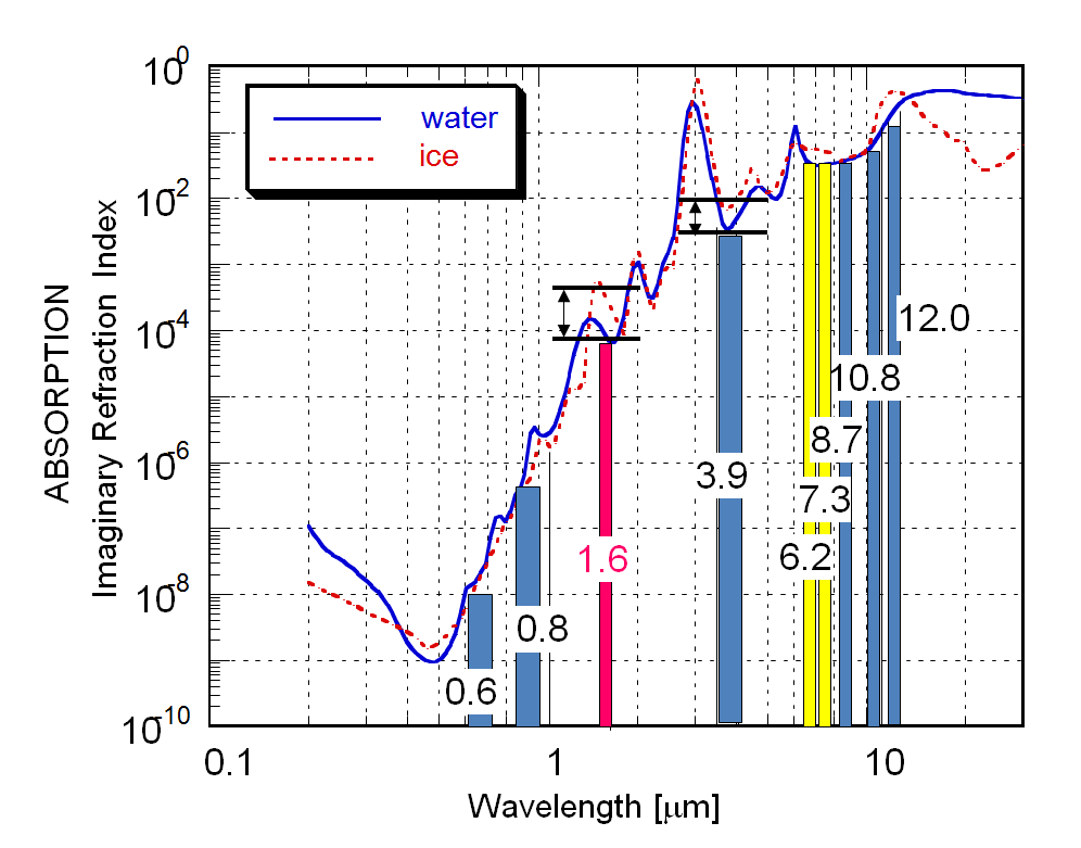
Discrimination of water and ice clouds is possible because the absorption is stronger for ice than for water both at 1.6 and the 3.9 µm wavelengths (Fig. 2). Due to the stronger absorption of ice the reflectivity of the ice clouds will be (usually) lower than that of the water clouds.
| Figure 2: Absorption spectra of water (blue curve) and ice (dashed red curve) and the spectral bandwidth of the SEVIRI channels. (Courtesy of Daniel Rosenfeld, HUJ) |
|
Creating Snow RGB images
The Snow RGB is composed of the VIS0.8, NIR1.6 and the 3.9 micrometer channel (IR3.9) data (Table 1). The measured values should be calibrated to calculate reflectivity (including also solar zenith angle correction). During daytime the IR3.9 radiance includes reflected solar contribution as well as emitted thermal radiation. In the Snow RGB we are interested only in the solar component. To create the snow RGB one has to calculate the solar component of the measured IR3.9 signal. The abbreviation IR3.9refl (in Table 1) indicates the reflectivity computed from the solar component of the measured IR3.9 radiation.
Table 1: 'Recipe' of the Snow RGB
| Colour beam | Channel | Range [%] | Gamma | |
|---|---|---|---|---|
| Red | NIR1.6 | 0 | 100 | 1.7 |
| Green | NIR1.6 | 0 | 70 | 1.7 |
| Blue | IR3.9refl | 0 | 30 | 1.7 |
Table 1 shows which channels (channel derivative) are visualised in the red, green and blue colour beams. Before combining them, these images should be enhanced in two steps. First a linear stretch is performed within the reflectivity ranges shown in the third and forth columns of the table. Then a so-called gamma correction (a nonlinear expansion) is used to enhance the contrast in the darker parts of the image. The 'Gamma' parameter of this correction is listed in the fifth column of the table.
The following example shows how the Snow RGB is combined from the VIS0.8, NIR1.6 and IR3.9refl images. The different steps of the enhancement are presented to show how the resulting RGB improves.
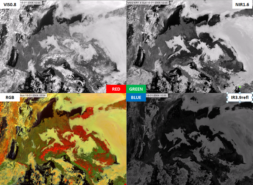
| Figure 3a: VIS0.8 (upper left), NIR1.6 (upper right), IR3.9refl (below right) images (all stretched within the 0-100 % reflectivity range) and the RGB created from these components (below left) for 15 January 2006 at 10:55 UTC |
|
Fig. 3a shows the VIS0.8, NIR1.6 and IR3.9refl images all visualized within the 0-100 % reflectivity ranges. The NIR1.6 image is darker than the VIS0.8 image and the IR3.9refl image is even darker. This is in accordance with Fig. 2 showing that the absorption of ice and water are much higher at 1.6 than at 0.8 micrometer and even higher at 3.9 micrometer. As a consequence the 0-100 % range seems to be NOT adequate for all three channels. For example, the blue channel seems to be too dark with this enhancement.
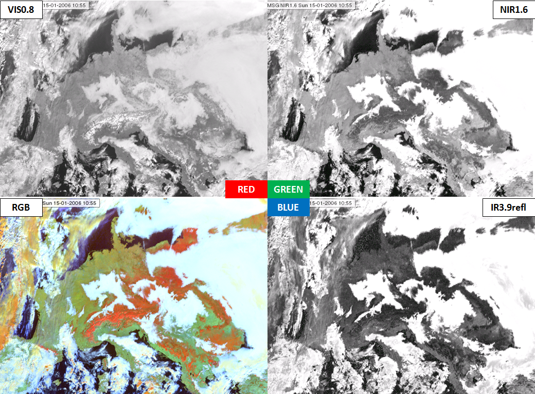
Fig. 3b shows the same images linearly stretched within the reflectivity ranges indicating in Table 1. The blue and the green colour components became brighter with the modified ranges. However, the snowy and snow-free land areas are not separated clearly enough in the IR3.9refl image.
| Figure 3b: VIS0.8 (upper left), NIR1.6 (upper right), IR3.9refl (below right) images, all stretched within the reflectivity ranges indicated in Table 1, and the RGB created from these components (below left) for 15 January 2006 at 10:55 UTC |

|
Fig. 3c shows the VIS0.8, NIR1.6 and IR3.9refl images enhanced according to the recipe of Table 1 (first linearly stretched and then gamma corrected). The snowy and snow-free land areas are separated clearly in the IR3.9refl image after the gamma correction.
| Figure 3c: VIS0.8 (upper left), NIR1.6 (upper right), IR3.9refl (bottom right) images, all stretched within the reflectivity ranges indicated in Table 1 and then gamma corrected, and the Snow RGB (bottom left) for 15 January 2006 at 10:55 UTC |
|
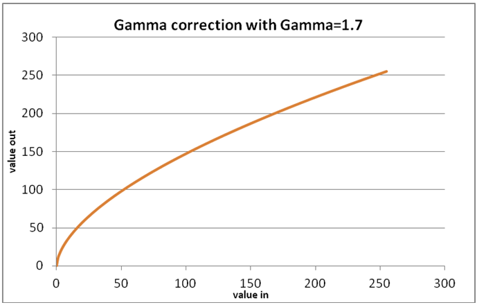
Why perform gamma correction? If a non-linear expansion is required, then gamma correction is performed after the linear stretching. The gamma correction enhances the contrast in the darker or in the brighter tones, depending on the Gamma parameter. In case of the Snow RGB (where Gamma is equal to 1.7), the contrast of the darker parts are increased, see Fig. 4.
| Figure 4: Effect of the gamma correction if the Gamma parameter is equal to 1.7 |
|
The bottom left panels of Figs. 3a, 3b and 3c show the RGB images created from the components presented on the corresponding figures. The bottom left panel of Fig. 3a shows the RGB when the components were linearly stretched in the 0-100 % reflectivity range. The bottom left panel of Fig. 3b shows the RGB when the components were linearly stretched in the ranges listed in Table 1. The bottom left panel of Fig. 3c shows the RGB when the components were first linearly stretched in ranges listed in Table 1, and then the gamma correction was applied. The last one is the Snow RGB. A comparison of these images shows how the RGB improves with proper enhancement.
Typical Colours of Snow RGB
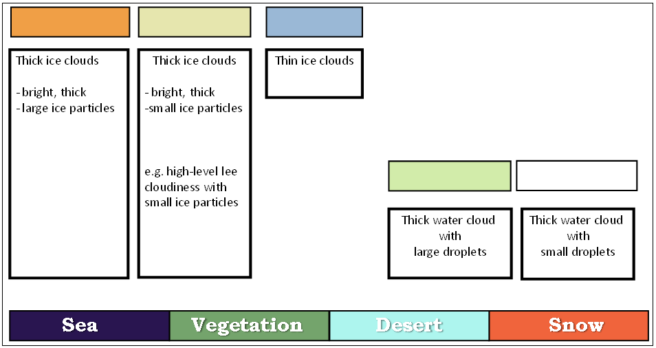
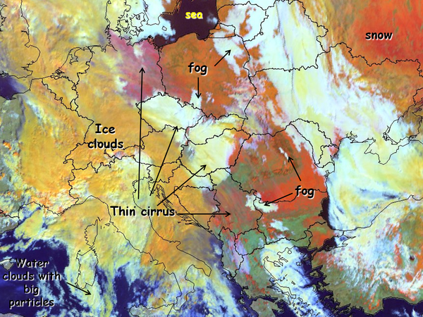
Water clouds are bright in all three components. Ice clouds are bright in the red one, gray in the green one and dark in the blue one. Snow cover is bright in the red component and dark in the green and blue ones. As a consequence the following colours will be typical for surface and cloud features (see Fig. 5):
- water clouds - white
- thick ice clouds - orange
- snow - red - orange
- vegetation - greenish
- desert - light blue
- sea - dark blue
- thin ice clouds - the colour depends on the colour of the underlying surface (sea, land or cloud) as well. For example, it could be pale bluish over sea or light yellowish over water clouds
| Figure 5: Typical Colours of Snow RGB (Source: Jochen Kerkmann, MSG Interpretation Guide, EUMETSAT) |
|
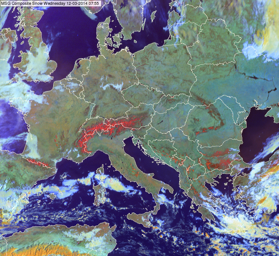
Several colours of the snow RGB are close to the natural colours: most of the water clouds are whitish, land is greenish and sea is dark blue (Fig. 6). There are also some non-natural colours: thick ice clouds are orange, snow is red-orange and the desert is bluish.
| Figure 6: Snow RGB for 12 March 2014 at 07:55 UTC |
|
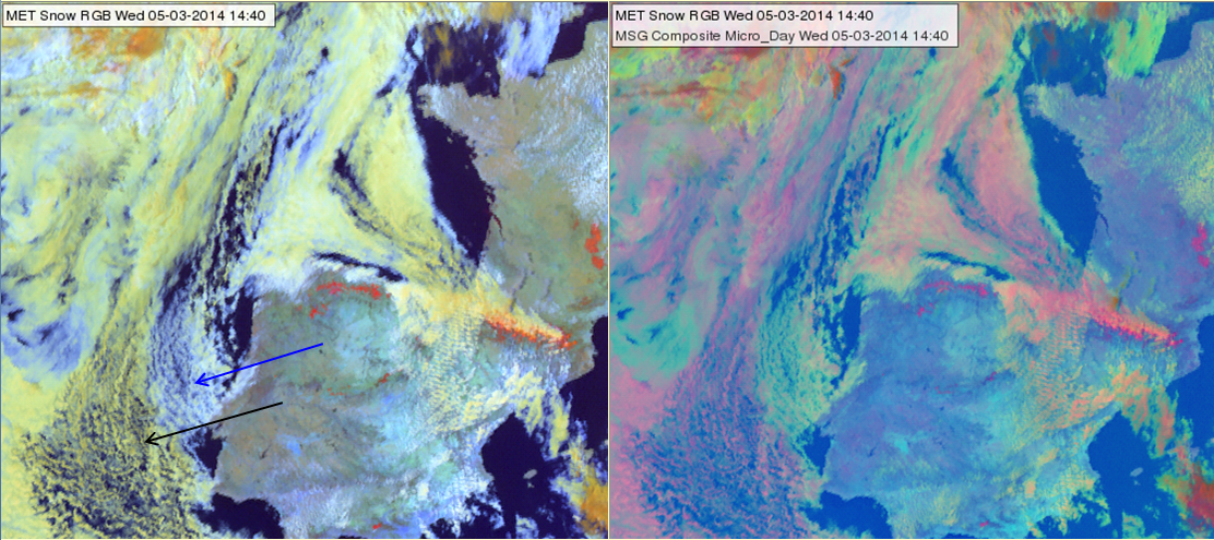
Note that the colour of the clouds depends slightly on the cloud top particle size as well, because the reflectivity of the clouds depends on their cloud top phase and particle size both in NIR1.6 and in NIR3.9 channels. Water clouds with large particles or ice cloud with small particles may have similar colours - pale yellowish green. Water clouds with big particles are depicted in a light greenish yellow, while water clouds with small particles appear white (see left panel of Fig. 7). The right panel of Fig. 7 shows the corresponding Day Microphysics RGB image.
| Figure 7: Snow RGB (left) and Day Microphysics RGB (right) for 5 March 2014 at 14:40 UTC. The blue and black arrows indicate water clouds with small and large particles, respectively. |
|
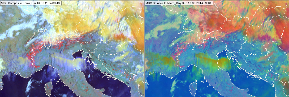
Ice clouds with big particles are orange, while ice clouds with small particles are light/pale yellow (with some greenish tones). Fig. 8 shows high-level lee clouds south and southwest of the Alps. High-level lee clouds typically consist of very small ice crystals.
| Figure 8: High-level lee clouds with small ice particles in the Snow RGB (left) and Day Microphysics RGB (right) south and southwest of the Alps for 16 March 2014 at 09:40 UTC |
|
Examples of interpretation
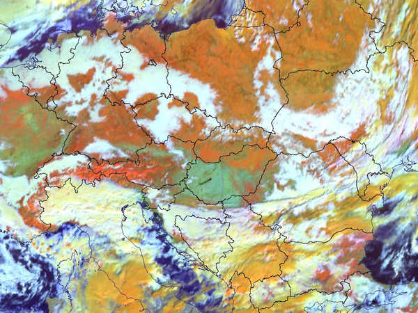
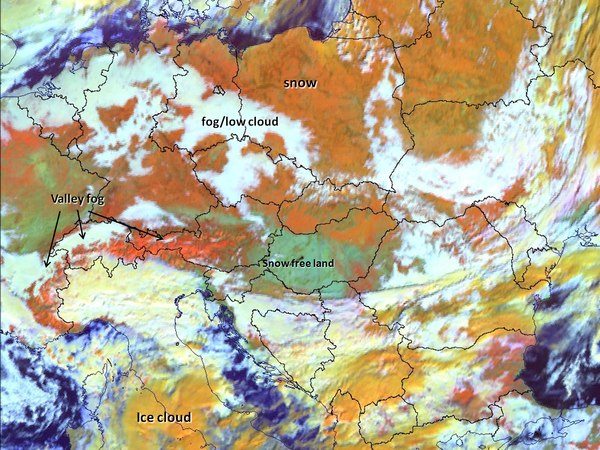
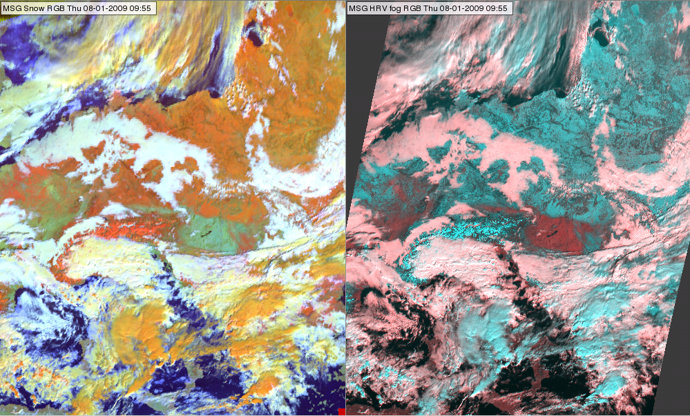
Two cases are shown with and without annotations to give examples on the proper interpretation of the different surface and cloud types in the Snow RGB images (Figs. 9 and 10). The valley fog in the Alps shows clearly in Fig. 9 because of the good colour contrast.
| Figure 9: Snow RGB with and without annotations for 08 January 2009 at 09:55 UTC |
|
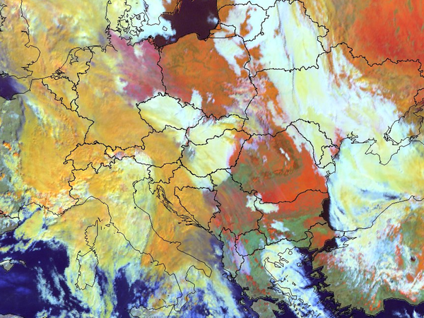
| Figure 10: Snow RGB with and without annotations for 05 February 2010 at 09:25 UTC |
|
The thin cirrus clouds across Germany, Hungary and Serbia are hard to see in Fig. 10.
Cloud-free snowy mountains and land can have different appearance in the satellite imagery. If the snow lies on a plain or low hill, one can often see patches, lines or spots in it. Patches might be due to forest with shadows and branches not covered by snow. Lines might be due to rivers, and spots (small patches) due to settlements. In mountainous terrain one can often see the structure of the valleys and ridges. Snow on high mountains is usually depicted in a brighter colour than on plains or hills, as there is less vegetation in the mountains to disrupt the snow cover.
Comparisons with other image types
Comparison with a single channel image
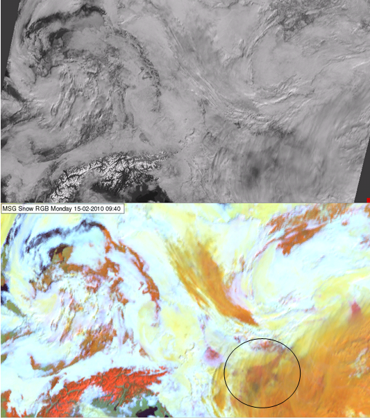
Fig. 11 compares a Snow RGB with an HRV image. The different features are much easier to recognize in the Snow RGB, although HRV has a better spatial resolution, which makes it easier to see the small-scale structure. However, in the black and white HRV image many objects are of similar brightness - the clouds, the snow, etc. The benefits of the RGB image are quite evident, such as in the encircled area. Here we see mainly snow covered surface through a hole in the water clouds through a thin cirrus layer. All these features are not easy (if even possible) to identify in an HRV image.
Distinguishing between water and ice clouds in HRV images might be even more problematic than distinguishing between snow and clouds. In a Snow RGB the ice and water clouds are easily separable: whitish colours indicate water clouds, while orange indicate ice clouds.
| Figure 11: HRV (top) and Snow RGB (bottom) images for 15 February 2010 at 09:40 UTC. |
|
Comparison with HRV Fog RGB
The main aim of Snow and HRV Fog RGBs is the same: differentiating cloud-free snowy surfaces from water clouds or fog. The spatial resolution is better for HRV Fog RGB, while the ice cloud / snow colour contrast is better in Snow RGBs (see for example Fig 12a). The benefits of high resolution are more evident when looking at a smaller area. Fig 12b shows a closer look at the Alps.
| Figure 12a: Snow RGB (left) and HRV Fog RGB (right) for 08 January 2009 at 09:55 UTC |
|
| Figure 12b: Snow RGB (left) and HRV Fog RGB (right) for 08 January 2009 at 09:55 UTC |

|
Exercise
Exercise
Question
Please, match the following cloud and land features to the numbers.
Thick ice clouds, Tin ice clouds / cirrus, Water cloud, Cirrus, Snow on mountains, Snow on mainland, Snow free land, Sea, Desert
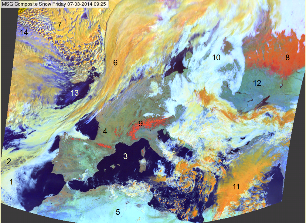
| 1 | 2 | 3 | 4 | 5 | 6 | 7 | 8 | 9 | 10 | 11 | 12 | 13 | 14 | |
|---|---|---|---|---|---|---|---|---|---|---|---|---|---|---|
| Tick ice clouds | X | X | X | |||||||||||
| Thin ice clouds / cirrus | X | X | ||||||||||||
| Water clouds | X | X | X | |||||||||||
| Snow on mountains | X | |||||||||||||
| Snow on mainland | X | |||||||||||||
| Snow free land | X | X | X | |||||||||||
| Sea | X | |||||||||||||
| Desert | X |