Recognition and Impact of Vorticity Maxima and Minima in Satellite Imagery

Introduction

Vorticity patterns control the circulation of air masses in their vicinity. By doing this they control the location of important meteorological quantities that are essential for an accurate diagnosis and forecast of the atmosphere.

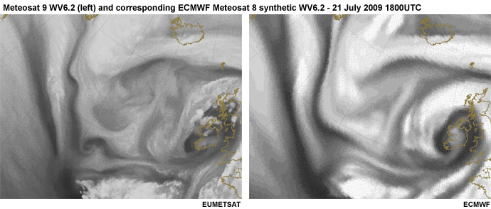
The scale of vorticity patterns in the atmosphere ranges from large-scale synoptic system circulations (low and high pressure centres) to smaller meso-scale circulations (water vapour vortices (sometimes referred as WV eddies or WV eyes). The (anti-)cyclonic rotation in the atmosphere caused by a vorticity maxima is easily seen in satellite imagery. And quite naturally, satellite imagery is the key tool to correctly locate the maximum of cyclonic and anticyclonic vorticity in the atmosphere. Moreover, satellite images are able to show the small-scale vorticity patterns that are easily overlooked and smoothed out by a NWP model. An example of this you see in the satellite images below where a range of small scale eddies resulting from a shear zone over the Atlantic Ocean were not recognised by the ECMWF model.

Meteosat 9 WV image compared to ECMWF synthetic water vapor

This training module has been developed to teach you to identify these vorticity centres in Meteosat Second Generation (MSG) satellite imagery. In addition the module will provide you with a firm physical background to help you understand why it is important to do a good diagnosis of satellite images and also provide you with a range of examples and exercises to demonstrate the impact a vorticity centre may have on your weather forecast.

To help refresh your memory, this first chapter will continue by presenting you the basics of vorticity by answering the question on "What is vorticity?". If you would already know the answer to this question you may choose to continue to chapter two on vorticity maxima.

What is Vorticity

Vorticity (which is expressed as ζ) is a measure of the rotation of fluids about a vertical axis relative to the earth's surface. In the northern hemisphere it is defined as positive or cyclonic in the counterclockwise direction. The unit of measurement of vorticity is inverse seconds (s^-1). The following two equations are identical:

Where U and V are the east and northward wind components of the wind velocity. R is the radius or curvature travelled by a moving air parcel, M is the tangential speed along that curve in a cyclonic direction, and n is the direction pointing inward toward the centre of curvature.

In the above equation you see the small subset r, which stands for relative. In these equations we do not take into account the rotation of the earth and therefore consider relative vorticity. A physical interpretation of the first equation can be seen in this animation.

Cyclonic vorticity induced on a small paddle as a result of windshear.

If fluid flows along a straight channel, and is bound by shear, then it also has vorticity because a tiny paddle would be seen to rotate.

The second equation is interpreted below, where fluid along a curved path also has vorticity, so long as radial shear of the tangential velocity does not cancel it.

Vorticity for flow around a curved path where both the curvature and shear contribute to positive vorticity.

A special case of the last equation is where the radial shear is just great enough so that winds at different radii sweep out identical angular velocities about the centre of curvature. In other words, the fluid rotates as a solid body. For this the last equation reduces to:

Below we see a maximum of cyclonic vorticity north of the wind maximum and a maximum of anticyclonic vorticity south of the wind maximum, as is recognised by the rotating paddle wheels. The lower of the two paddles will turn clockwise (anticyclonic) since the wind force on the northern side of the blades is stronger than the force on the blades south of the axes.

Two dimensional flow with linear shear resulting in cyclonic and anticyclonic vorticity centers.

For this fact the poleward and equatorward sides of a westerly jet are always referred to as the cyclonic and anticyclonic shear sides, respectively.

Absolute Vorticity

The absolute vorticity is the sum of the relative vorticity and the earths' rotation.

where f_c is the coriolis parameter f_c = 2 Ω sin (Φ) and is a measure of the velocity of the earths' rotation.

Potential Vorticity

Potential vorticity ζ_p is defined as the absolute vorticity divided by the depth Δz of the column of air that is rotating.

It has units of m^-1 s^-1. In the absence of turbulent mixing and heating (latent radiation), potential vorticity is conserved (i.e. remains constant).

Isentropic Potential Vorticity

The Isentropic Potential Vorticity (IPV) can be defined as:

Where ζ_p is the potential vorticity measured on an isentropic surface (i.e. a surface connecting points of equal potential temperature θ) and where ρ is the air density (e.g., 1.2 kg m^-3)

By rewriting the above equation as:

we can derive that larger IPVs exist where the air is less dense and where the static stability Δθ / Δz is greater. For this reason, the IPV is two orders if magnitude greater in the stratosphere than the troposphere. IPV is measured in potential vorticity units (PVU) defined by 1 PVU = 10^-6 K m² s^-1 Kg^-1. On average the air in the troposphere ζ_IPV <1.5, while in the troposphere this is greater.

Isentropic Potential Vorticity is conserved for air moving adiabatically and without friction along an isentropic surface (i.e., a surface of constant potential temperature). Thus, it can be used as tracer of air. Stratospheric air entrained in the troposphere retains its IPV>1.5 PVU for a while before losing its intensity due to turbulent mixing.

Vorticity Advection

One parameter that is often presented on weather maps is positive vorticity advection, or PVA. This is a parameter widely used to explain the concept of cyclogenesis but can be a bit harder to understand. The following animation is designed to simplify the processes leading up to PVA and what effect it has on the weather.

Cyclonic Vorticity and Comma Patterns

Season: Every day
Phenomena: Moist Circulations, Vorticity Maxima and Vorticity Advection
Tools: Meteosat Second Generation: WV6.2 and Airmass RGB

Forecast Challenges:

Identify and predict the vorticity maxima in order to predict areas of positive vorticity advection
Identify the related axes of maximum winds, deformation zones and air masses
Isolate what impact of the vorticity maxima will have on your forecast

Vorticity maxima signatures are very common and indicate areas of ascending circulation and atmospheric forcing. The correct placement of the maximum of cyclonic vorticity is vital to the placement of related dynamic features such as the axis of maximum winds and deformation zones.

Note: All examples and conceptual models in this module are set in the northern hemisphere. All graphics are oriented north to south with north on top.

Development of a Comma Pattern

The shape of the cyclonic comma pattern helps immediately to reveal the location of the vorticity maximum. This is illustrated in animations below. In the animations you can recognise the shape of two arches representing inflow (concave) and outflow (convex). The shape of these arches are related to both the intensity of the vorticity maximum and to the length of time the vorticity maximum has been acting on these arcs. The point of intersection of these two arches is called cusp and is the location of the cloud rotation and the vorticity maximum.

The vorticity maximum (X) is the addition of both horizontal wind shear (S) (simply referred to as shear hereafter) and rotational vorticity (R). The following graphics illustrate the concept. The size of the symbols indicates their relative intensity.

Given pure rotation, this conceptual cloud line will evolve in a symmetrical fashion. The position of the vorticity maximum (X) is at the center of the rotation, which is in this case also the cusp (the point where two curves intersect). The rotational vorticity (R) is the sole component of vorticity. There is no shear vorticity component. The shape of the comma is then determined by both the intensity of the vorticity maximum and its age. Please note that situations like this you will not often find in your daily operational work. Normally there is some increased shear component working on the rotation to act on the shapes of the in- and outflow arches.

The second animation reveals some differences from the first. On the equatorial side of the rotation there is increased shear (as marked by the bigger S), the cusp and by this the total vorticity is shifted towards that region of greater shear. The arc of inflow and the location of the wind maximum are enhanced. The outflow arc is not enhanced and is created purely by the rotational component of the vorticity, which remains unchanged and located at the center of the circle. The vorticity maximum (X), resulting from the sum of the rotational (R) and shear vorticities (S), is hereby thus shifted to the south! This pattern is very common due to the prevailing westerly circulations around the globe.

With even stronger winds the equatorial shear component of the vorticity increases and there is more displacement of the total vorticity and point of inflection toward the region of shear and away from the position of the rotational vorticity centre. The inflow arc in the location of the wind maximum is really enhanced. And again, with increased shear vorticity, the vorticity maximum will also be much more intensive.

Another scenario takes place when we place the shear on the poleward side of the rotation, the same shifting of the cusp and the vorticity maximum takes place, again with the center of total vorticity shifting towards the region of shear. In contrast, however, the convex arc in the location of the wind maximum is enhanced. The concave arc is not enhanced and is created purely by the rotational component of the vorticity, which remains unchanged and located at the center of the circle. The vorticity maximum will be buried within the moisture area as opposed to the previous illustrations, where it is located in the dry portion of the circulation. This enhancing of the convex arc is "vexing" in that the point of inflection and vorticity maximum may be more difficult to locate than when the vorticity is dominated by its rotational component or when the shear is equatorward of the rotational center.

Poleward shear comma shapes are common with the northeast trade winds in the tropics.

The four scenarios presented above showed variable strengths of shear vorticity on equator and poleward side and how these act on the formation of comma shapes. It is important that when using satellite images you are able to recognise the position of the vorticity maximum. This maximum is situated at the cusp, which is the intersection point of both the outflow and the inflow arch! Using an animation of several satellite images will significantly help you to identify whether shear is found on the poleward or on the equatorward side of the maximum.

Morphology of a Comma Pattern

Roger Weldon originally identified the "comma" cloud pattern in the early 1980's. The cloud and absolute vorticity isopleth correlations he used were empirical. Variation in cloud heights from 500 hPa and time differences between the analysis and the satellite data can lead to errors. However, the centre of cloud rotation as identified by the cusp and the point of inflection is the vorticity maximum.

Comma Dominated by Rotation and/or Equatorial Shear

The inflow arc is associated with the jet axis and defines this type of comma. The portion where you find the maximum of inflow identifies where the jet axis crosses into the moisture area.

Conceptual model dominated by equatorial shear

The comma head is the portion of the comma downstream from the vorticity maximum. Positive vorticity advection will be strongest in the comma head region as this enhancement is related to the left exit region of the jet.

Comma Dominated by Poleward Shear

The convex arc defines this type of comma. The concave arc region is minimal, and the point of inflection is buried within the moisture area. The comma head is still that portion of the comma downstream from the vorticity maximum.

Conceptual model dominated by poleward shear

Other Considerations

With both patterns, the comma tail is associated with the warm conveyor belt. Vorticity advection will be minimal in this region. The comma tail begins at the upstream long wave trough.
It is very important to remember that all satellite features are generated by system-relative motions.
If moisture elements on the poleward side of the cyclonic circulation are stationary or moving westward with respect to the earth's surface, the vorticity maximum is actually a closed upper low or cold core low.

Analysis

In the following interaction, first take a look at the MSG WV6.2 and Airmass loop, then analyze it for the axes of maximum winds, vorticity maxima, and vorticity minima. After identifying these features, compare your analysis to the one provided by the expert.

Interpretation

Geopotential Height 300 hPa.

Meteosat 9 WV6.2 and ECMWF 300 hPa Geopotential Heights

The most striking feauture in the loop was the rapid development of a depression south-west of Iceland. In this image the geopotential height (cyan) is compared to the deformation zones (green). As for the Rapid Cyclogenesis near Iceland, no strong signal is seen yet in the upper layers (as you would expect). A marked trough identifies the development. A second remarkable trough is found over the UK. The deformation zones indicate two vorticity maxima captured by a sharp upper level trough.

In between the Rapid Cyclogenesis and the upper level trough over the UK a broader deformation zone is found west of Ireland. The geopotential height shows some weak upper level trough. Quasi geostrophic forcing could be associated with this and one should monitor this accordingly.

Isotachs and PVA 300 hPa.

Meteosat 9 WV6.2 and ECMWF 300 hPa Isotachs and PVA

Several wind maxima are found in the image. One is seen over the Atlantic west of Spain and France associated with the anti-cyclone over the Azores. A second wind maximum is found over England and the North Sea. The most important wind maximum is found over the Atlantic and is associated to our Rapid Cyclogenesis system. The development of this system is taking place in the left exit region of the Jet. In orange, a pronounced PVA maximum can be witnessed. Further development of this system to a mature depression may still be expected.

Height of PV equals 1

Meteosat 9 WV6.2 and ECMWF 300 hPa Height of PVA equals 1

The height (in pressure) at which the potential vorticity (PV) equals 1 PV units (10^-6 m^-2 s^-1 K kg^-1) is plotted in this image in magenta. A pretty decent match is found with the vorticity maxima that are found by our "Expert". Especially when looking at Rapid Cyclogenesis the quick developments taking place can sometimes be misinterpreted by the model (e.g. model being too slow or too fast or diganosing a wrong track for the cyclone). Your knowledge of the water vapour images and its interpretation can then make a difference and help you to prefer one model over the other. In this case the PV anomaly South-West of Iceland is diganosed correctly in shape. The maximum would however be expected to be found near the cusp as opposed to where it is found now (more south) by the ECMWF +18 hour forecast.

Relative Vorticity 500 hPa.

Meteosat 9 WV6.2 and ECMWF 500 hPa Relative Vorticity

The relative vorticity in 0.5° resolution of ECMWF is plotted in this image. The small scale vortices are not being picked by the model (obvious because of the model resolution). Again it can be observed that the diagnosis of the Rapid Cyclogenesis South-West of Iceland is a bit too fast by the model. The true maximum as indicated by the cusp and by the X in this image is found more to the NNW. These things are important and can help you to prefer one model over the other. The important questions the forecaster has to deal with when forecasting the evolution of Rapid Cyclogenesis like this are:

Is the deepening rate of the low pressure centre in accordance with the reality?
Will the low pressure take the track as suggested by the NWP?
What will the changes in the forecast be if there are signs of model inconsistencies?

These questions have also lead to some research in European Weather Services in which the information from (potential) vorticity is changed after interpretation of the WV images. The technique, which is known as PV inversions, can help to improve the forecast and help in forecasting high impact weather more correctly. It has to be pointed out that changing PV field subjectively with the satellite image information is not a straightforward process, and it can also lead to erroneous interpretations, and great care has to be taken when applying PV inversion techniques in operational forecasting.
The method briefly can be summarised as follows:

Possible mismatches between the PV field in the analysis and features in the WV imagery are identified.
PV is modified at sensitive levels, based on shear vorticity information. Modified initial state is "tuned" to fit observations.
PV inversion is carried out.
The model is re-run from the modified initial state.

Implications

The correct placement of vorticity maxima is vital to the placement of related dynamic features such as the axis of maximum winds and deformation zones. All of these dynamic features must fit cohesively into the atmospheric puzzle. The correct placement of a vorticity maximum might be the piece of the puzzle required to correctly identify and place other dynamic features.

Here are some important attributes of vorticity maxima to keep in mind when identifying them:

Circulations around vorticity maxima are typically strong. As a result, numerical analyses of the atmosphere are typically successful in their placement and appropriate relative intensity. However, if numerical analyses should misplace or not analyze a vorticity maximum, the implications on the predictions could be important.
Cyclonic circulations tend to be rather moist.
Correctly identifying and locating vorticity maxima can help better predict convection and cloud patterns.
Convective feedback in numerical models can generate spurious vorticity maxima that can be identified as inappropriate through a careful analysis of the WV imagery.
The use of the Airmass RGB can have both strenghts as weaknesses. The strength is that it reveals the 3D aspect of the atmosphere. The weakness is that you must remember that the atmosphere and the dynamic features are 3D as well, so vorticity centres are actually vorticity tubes that are not necessarily vertical. This applies to all dynamic features.

Vorticity Maxima Exercise

The following exercises present you with 25 three-hourly WV6.2 images from October 2007. We want you to especially concentrate on the depression that you see located west of Ireland. For this first image click the position where you think the Vorticity Maximum is found. When done click the '+' and move three hours ahead in time to do the same again. When finsihed you may click the 'expert analysis' to compare your results.

Vorticity Minima and Anticomma Patterns

Season: Every day
Phenomena: Dry Circulation, Vorticity Minima, and Vertical Velocity
Tools: Meteosat Second Generation: WV6.2 and Airmass RGB

Forecast Challenges:

Identify and predict vorticity minima in order to predict areas of negative vorticity advection
Identify the related axes of maximum winds, shear zones, deformation zones, and air masses

Vorticity minima signatures are every bit as common as vorticity maxima signatures. They indicate areas of descending circulation and atmospheric forcing and can be used to diagnose dynamic features such as the axis of maximum winds and deformation zones.

Note: All examples and conceptual models in this module are set in the northern hemisphere. All graphics are oriented north to south with north on top.

Development of a Comma Pattern

The shape of the anticyclonic comma pattern helps immediately to reveal the location of the vorticity minimum. This is illustrated in animations below. In the animations you can recognise the shape of two arches representing inflow (concave) and outflow (convex). The shape of these arches are related to both the intensity of the vorticity minimum and to the length of time the vorticity minimum has been acting on these arcs. The point of intersection of these two arches is called cusp and is the location the cloud rotation and the vorticity minimum.

The vorticity minimum (N) is the addition of both horizontal wind shear (S) (simply referred to as shear hereafter) and rotational vorticity (R). The following graphics illustrate the concept. The size of the symbols indicates their relative intensity.

Given pure rotation, this conceptual cloud line will evolve in a symmetrical fashion. The position of the vorticity minimum (N) is at the center of the rotation, which is in this case also the cusp (the point where two curves intersect). The rotational vorticity (R) is the sole component of vorticity. There is no shear vorticity component. The shape of the comma is then determined by both the intensity of the vorticity minimum and its age. Please note that you will not often find situations like this in your daily operational work. Normally there is some increased shear component working on the rotation to act on the shapes of the in- and outflow arches.

The second animation reveals some differences from the first. On the equatorial side of the rotation there is increased shear (as marked by the arrow), the cusp and by this the total vorticity is shifted towards that region of greater shear. The arc of inflow and the location of the wind minimum are enhanced. The outflow arc is not enhanced and is created purely by the rotational component of the vorticity, which remains unchanged and located at the center of the circle. The vorticity minimum (N), resulting from the sum of the rotational (R) and shear vorticities (S), is hereby shifted to the south! This pattern is very common due to the prevailing westerly circulations around the globe.

With even stronger winds the equatorial shear component of the vorticity increases and there is more displacement of the total vorticity and point of inflection toward the region of shear and away from the position of the rotational vorticity centre. The inflow arc in the location of the wind maximum is really enhanced. And again, with increased shear vorticity, the vorticity minimum will also be much more intensive.

Another scenario takes place when we place the shear on the poleward side of the rotation, the same shifting on the cusp and the vorticity minimum takes place, again with the center of total vorticity shifting towards the region of shear. In contrast, however, the convex arc in the location of the wind minimum is enhanced. The concave arc is not enhanced and is created purely by the rotational component of the vorticity, which remains unchanged and located at the center of the circle. The vorticity minimum will be buried within the moisture area as opposed to the previous illustrations, where it is located in the dry portion of the circulation. This enhancing of the convex arc is "vexing" in that the point of inflection and vorticity minimum may be more difficult to locate than when the vorticity is dominated by its rotational component or the shear is equatorward of the rotational center.

Poleward shear comma shapes are common with the northeast trade winds in the tropics.

The four scenarios presented above showed variable strengths of shear vorticity on equator and poleward sides and how these act on the formation of anticomma shapes. It is important that when using satellite images you are able to recognise the position of the vorticity minimum. This minimum is situated at the cusp, which is the intersection point of both the outflow and the inflow arcs! Using an animation of several satellite images will significantly help you to identify whether shear is found on the poleward or on the equatorward side of the minimum.

Morphology of an Anticomma Pattern

Roger Weldon originally identified the "comma" cloud pattern in the early 1980's. The anticomma pattern is a mirror interpretation of that. Weldon showed correlations between the clouds, streamlines, and absolute vorticity isopleths. Note that absolute vorticity isopleths are used as an operational surrogate for system relative streamlines. Variation in cloud heights from 500-hPa and time differences between the analysis and the satellite data can lead to errors. The centre of cloud rotation, as identified by the point of inflection, is the vorticity minimum to a very close operational approximation.

Anticomma Dominated by Rotation and/or Equatorial Shear

The concave arc associated with the shear wind maximum defines this type of anticomma. The anticomma head is downstream from the vorticity minimum. Negative vorticity advection will be strongest in the anticomma head region.

Conceptual model of an anticomma dominated by equatorial shear

Anticomma Dominated by Poleward Shear

The convex arc associated with the poleward wind maximum defines this type of anticomma. The concave arc region is minimal and the point of inflection is within the moisture area. The anticomma head is still downstream from the vorticity minimum.

Other Considerations

With both patterns, the anticomma tail is associated with the warm conveyor belt. Vorticity advection will be minimal in this region. The anticomma tail begins at the upstream long wave trough.
It is very important to remember that all satellite features are generated by system relative motions. The anticomma pattern is identified by a general lack of clouds. Moisture patterns evident on the water vapour imagery may be the best, if not the only, means of locating them.
If moisture elements on the equatorial side of the anticyclonic circulation are stationary or moving westward with respect to the earth's surface, the vorticity minimum is actually a closed upper high.

Analysis

In the following interaction, first take a look at the MSG Airmass and WV6.2 loop, then analyze it for the axes of maximum winds, vorticity maxima, and vorticity minima. After identifying these features, compare your analysis to the one provided by the expert.