Water Vapour Imagery Pallet - Chapter V

Transverse cloud bands

Transverse cloud bands are often seen as substructures in high level cirrus cloud bands accompanying the subtropical jet stream. These fiber-like cloud bands are oriented perpendicular to the subtropical jet axis and consist of thin ice clouds. While the transverse cloud bands typically show lengths of dozens to hundreds of kilometers, the main cirrus cloud band can be 2000 km long or more (figures 1 and 2). The typical orientation of the subtropical jet cloud band is southwest to northeast. Similar to the polar front jet streak, the subtropical jet streak is also accompanied by a black stripe in WV imagery. In contrast to the polar front jet, the subtropical jet stream is restricted to temperature and WV gradients in the upper troposphere.

a)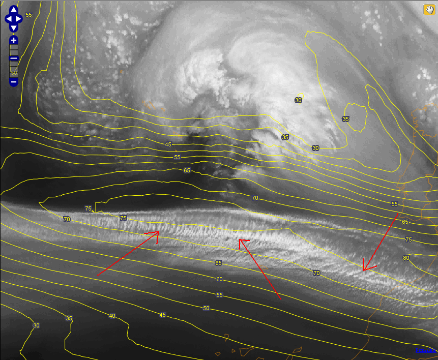

b)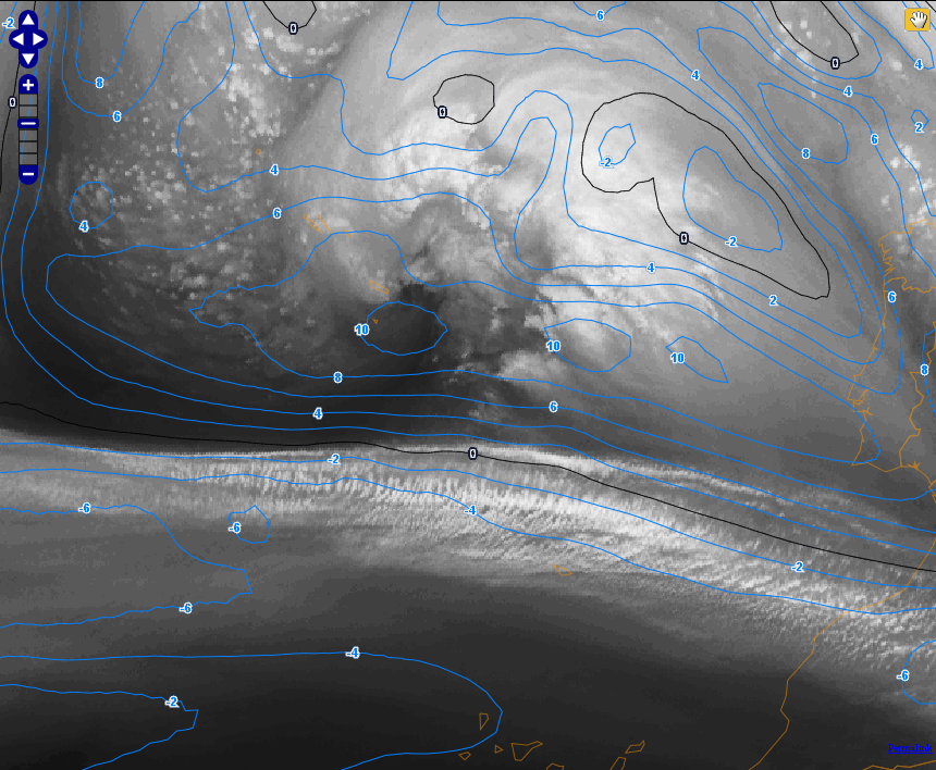

Figure 1a and 1b: Transverse cloud bands (red arrow) within a cirrus cloud band over the Atlantic in WV 6.2 µm imagery. Left image with isotachs at 300 hPa, right image with shear vorticity at the same level.

In satellite images, these transverse cloud bands have a similar appearance to lee waves at the lee of mountain ranges, but while the first can be detected in the WV channels, the latter usually cannot be seen in WV images as they are located in lower tropospheric regions.

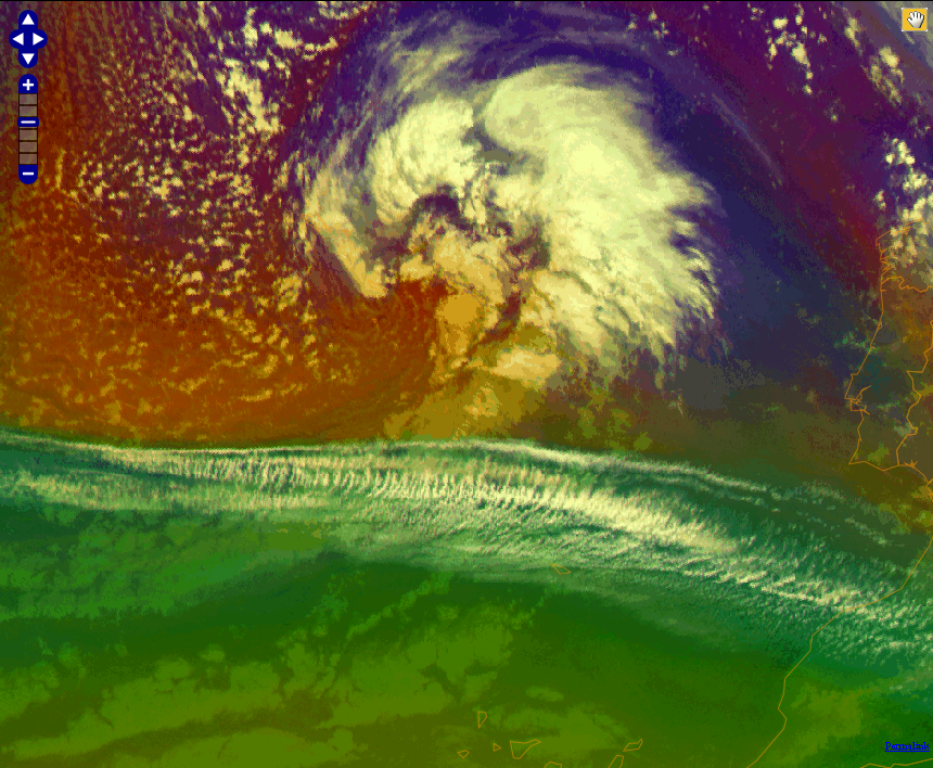
Figure 2: Same region as in figure 1 but in Air Mass RGB

The SEVIRI Air Mass RGB differentiates between cold and warm air masses. The green component shows the difference between MSG channels 9.7 and 10.8 microns. Channel 9.7 is responsive to ozone concentration in the lower stratosphere. In a warm air mass the tropopause is higher than in a cold air mass, and consequently the ozone concentration in the upper troposphere is smaller. This results in a more greenish colour than in a cold air mass, which appears in blue. In this image from 2 April 2013 at 06:00 UTC, there is a sharp boundary between warm and cold air masses. The jet core is running nicely along the border between the warm green and the cold reddish-bluish air masses. The reddish area north of the jet marks a dry zone with descending stratospheric air at the rear side of a cold front. For more information on the Air Mass RGB see chapter 9.

Kelvin-Helmholtz instability

The origin of transverse cloud bands lies in the vertical velocity shear caused by the subtropical jet stream. When wind shear increases (as is the case near the jet streak), frictional forces within the stable stratified air increase. Friction between layers with differing wind speed leads to small disturbances forming a wave-like pattern within the atmospheric stream, similar to the way wind interacts with an ocean's surface. When the air is near saturation, ice crystals form at the wave crest. This can be detected in satellite images. When the wind shear is strong enough, the Kelvin-Helmholtz waves will break (see figure 3) and lead to moderate or severe turbulence.

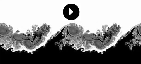
Figure 3: Numerical simulation of Kelvin-Helmholtz instability (source Wikipedia)

Notice:

Scallops

Kelvin-Helmholtz waves do not necessarily appear in vertical wind shear alone as is the case for transverse cloud bands. In fact, they can also be observed in WV imagery as horizontal waves (scallops) near the jet axis at the border of the cirrus cloud band accompanying the subtropical jet streak.

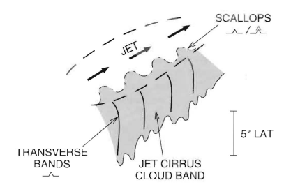
Figure 4: Schematic showing the relative position of turbulence to transverse bands and scallops in a jet cirrus cloud band. Dashed lines enclose regions where moderate turbulence is likely.

Scallops are formed by horizontal perturbations of a laminar air flow in regions of strong horizontal wind shear. These horizontal Kelvin-Helmholtz waves are visible because perturbations are generated at the intersection of the cirrus cloud shield and clear skies (figures 4 and 5). The edge of the cloud often appears ragged, sometimes with thicker, lumpy cloud parts.

Figure 5: MSG WV 6.2 µm satellite image from 11 April 2013 at 10:30 UTC. The red arrows show the scallop pattern over Spain and the Bay of Biscay.

Example: 22 October 2012, 12:00 UTC

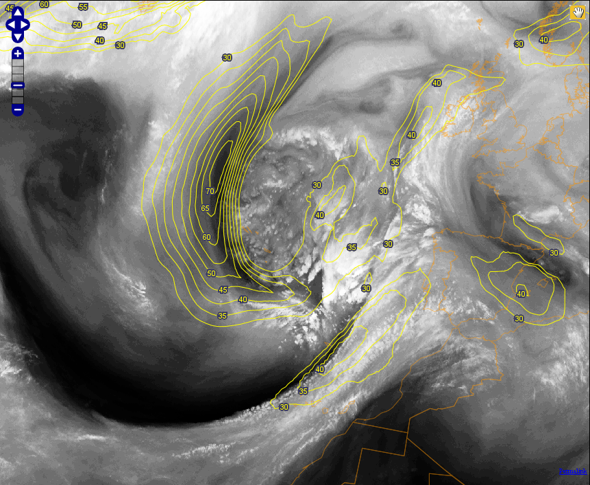
Figure 6: WV 6.2 µm image from 22 October 2012 at 12:00 UTC. The yellow isolines depict the isotachs [m/s] of the jet at 300 hPa.

The WV image from 22 October 2012, 12:00 UTC (figure 6) shows a branch of the polar jet stream over the Atlantic heading towards the southeast and a branch of the subtropical jet west of Morocco and Portugal heading towards the northeast. A dark stripe in the WV 6.2 µm image is clearly visible on the cold side of the jet axis for both jet streaks. The moisture gradient zone corresponds to the axis of the jet.

a)	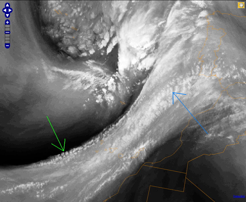b)
c)	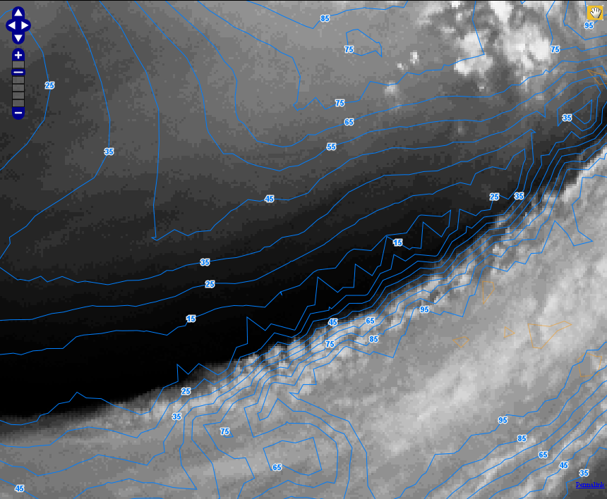d)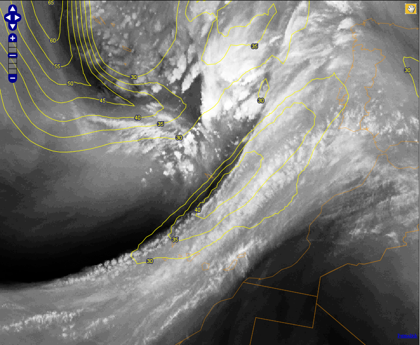

Figure 7a-7d: WV 6.2 µm image from 22 October 2012, 12:00 UTC
a) The WV 6.2 µm satellite image shows scallops at the back of a frontal cloud band (green arrow) and transverse cloud bands inside it (blue arrow).
b) WV 6.2 µm satellite image with shear vorticity isolines.
c) Isolines of the relative humidity [%] at 300 hPa.
d) Isotachs [m/s] at 300 hPa.

The WV satellite image of 22 October 2012 shows scallops near the axis of the subtropical jet and transverse cloud bands at the center and eastern parts of the frontal cloud band (figure 7a). The shear vorticity shows high values in this area at the 300 hPa level. A maximum of cyclonic shear vorticity, which favors the formation of scallops, can be distinguished along the dark WV stripe. In the middle of the cloud band there is a maximum of anticyclonic shear vorticity (negative sign), where transverse cloud bands can be seen.

A vertical cross section (figure 8a-8d) through the cloud band west of Morocco shows that the frontal zone is located above 600 hPa. This upper level cold front marks the transition from a dry stratospheric air mass to a warmer and more humid one. ECMWF cloud parameterization shows the presence of high level cloudiness above 500 hPa.

a)	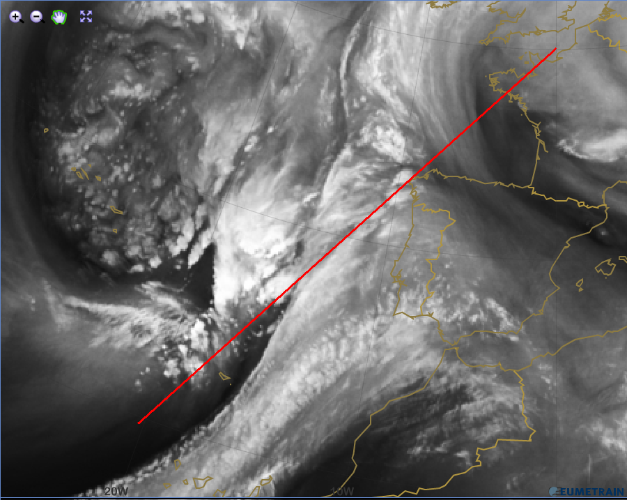b)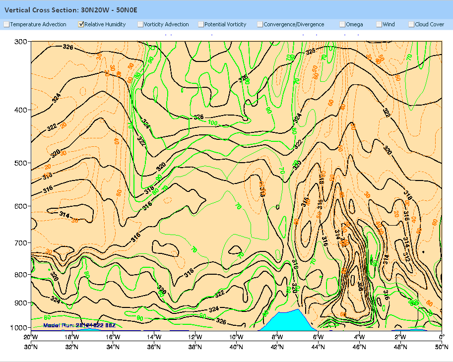
c)	d)

Figure 8a-8d: Vertical cross section through the upper level cold front with ECMWF model data. Date is the same as in figure 7.
a) Position of the vertical cross section (red line)
b) Equivalent potential temperature (black) and relative humidity (green/brown)
c) Equivalent potential temperature (black) and cloud cover (green)
d) Equivalent potential temperature (black) and isotachs (brown)

The isolines of the equivalent potential temperature in figure 8b-8c show the position of the upper level front between 16W/34N and 14W/36N. The cloud cover visible in satellite imagery is reflected in the model fields as well as the high values of relative humidity as a precondition for condensation. The isotachs suggest strong vertical wind shear.

This environment is favorable for Kelvin-Helmholtz waves to become visible in IR images, and in WV images they are even clearer. While descending air masses in the wave trough tend to warm up and evaporate cloud droplets/ice crystals, the moisture in the air condenses at wave crests. High values of relative humidity are necessary for the wave pattern to show up in satellite imagery.