Atmospheric Motion Vectors (AMV)
The technique of tracking features in time sequences of satellite images for estimating atmospheric motions is used since the 1970s. Since then, the coverage and quality has notably improved mainly because of higher resolved image data and better algorithms but also because of the availability of WV channels.
The advantage of using WV images is that the AMVs can also be detected in cloud free areas and that their features are more conservative in time than features in IR or VIS images. An example for such a product is the NWC-SAF's High Resolution Wind Product (HRW). It produces a high quality field of AMV.
How are AMVs derived?
First, the feature to be traced or a candidate target has to be selected. Some preconditions have to be met when selecting a tracer cloud:
- The feature must be large compared to the resolution of the images
- The life-time of the feature has to be longer than the time interval of the tracking sequence
The second step is to track the target in a time series of images in order to determine its motion relative to a fixed location, and consequently, the wind vectors. This is done by using either the “Euclidean distance” method or the “cross correlation” method.
The derived vectors have to be assigned to a height. This is one of the trickiest and error-prone operations/steps in the processing chain. To deduce whether the sky is cloudy or cloud-free, one has to determine the brightness temperature of the selected target and calculate the temperatures for its base and top.
With the help of a NWP forecast model or – if no model is available – a climatological profile, the temperature values are converted to pressure values. Another algorithm then determines which of the two pressure levels best represents the displacement. In clear air conditions the AMV-height is assigned by using the pressure level derived from the WV brightness temperature.
There are certain post-processing procedures that follow the processing of the AMVs. They will only be given a cursory explanation here. The first post-processing step is to assign a quality index to every vector. This quality index is computed by checking wind direction, speed and vector consistency while comparing them with those of previous images.
Consistency with neighboring vectors and NWP model wind fields is then factored in. The quality index is a weighted average over these temporal, spatial and forecast tests.
Orographic flag calculation is another post-processing procedure. This is done only for AMVs over land, and its purpose is to detect and reject vectors that are affected by the ground (e.g. orographic clouds).
Applications
AMVs are the only observations that provide a good coverage of upper tropospheric wind data over oceans and high latitudes. The observation and analysis of weather phenomena occurring in data-sparse regions will therefore profit from this data source.
Possible applications are:
- Tropical cyclones: AMVs are useful in depicting upper-level features. The data can also be used for forecasts or analyses and case studies. This means AMVs can help in understanding and forecasting a cyclone’s formation, intensity and track.
- AMVs can be used for analyzing meteorological conditions, especially over oceanic regions
- AMVs can be processed for assimilation into NWP models
- AMVs can be used for reanalysis of past synoptic situations
Figure 2 shows an example of AMVs computed by the SAF-NWC. The different colours denote different atmospheric levels. Changes in wind velocity and direction can be deduced from this product.
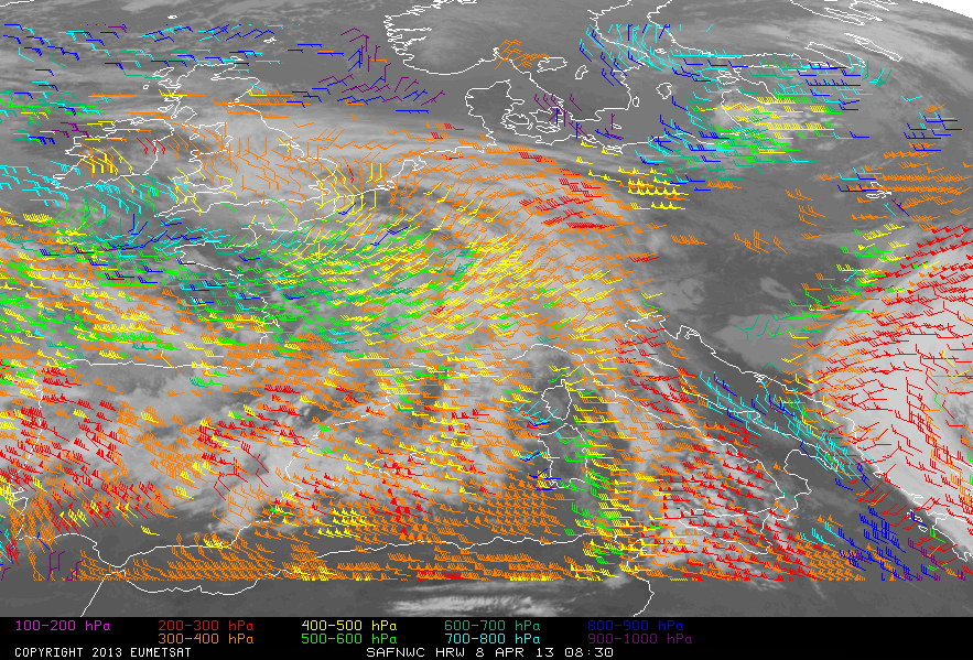
Figure 2: SAFNWC/MSG HRW AMVs for an area covering most of Europe and the Mediterranean: 08 April 2013 08:30 UTC (source: http://www.nwcsaf.org/)
Example: Hurricane Gordon
In September 2006 Hurricane “Gordon” first affected the Azores Islands as a hurricane and a few days later hit the north-western parts of the Iberian Peninsula as a tropical storm. In figure 3 the AMV analysis and the corresponding HRVIS satellite image of this date can be seen. The tropical storm is located in the south-western corner of the image connected to the southern end of a cold front. The surface low associated to Gordon can be detected quite clearly from the satellite image, but as the cyclone is completely embedded in the general flow of the cold front only a slight cyclonic deviation of the flow can be seen together with strong winds in lower layers.

Figure 3: HRVIS image and AMV analysis of the tropical storm Gordon, 21 September 2006, 14:30 UTC.
Question
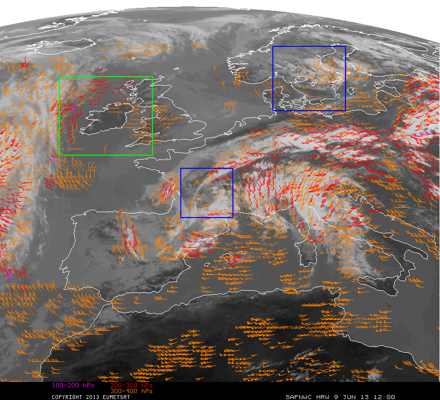
Find regions with upper level cyclonic and anticyclonic rotation.
- Solution: Click here to see these regions.